Transcription
Constraint Satisfaction ProblemsAIMA: Chapter 6CIS 391 - Intro to AI1
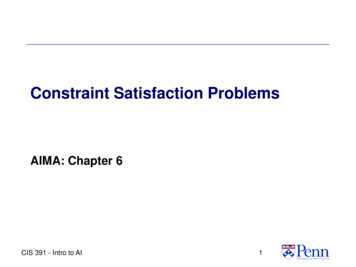
Constraint Satisfaction ProblemsA CSP consists of: Finite set of variables X1, X2, , Xn Nonempty domain of possible values for each variableD1, D2, Dn where Di {v1, , vk} Finite set of constraints C1, C2, , Cm—Each constraint Ci limits the values that variables can take,e.g., X1 X2 A state is defined as an assignment of values tosome or all variables. A consistent assignment does not violate theconstraints. Example: SudokuCIS 391 - Intro to AI2
Example: CryptarithmeticX3X2X1 Variables: F T U W R O, X1 X2 X3 Domain: {0,1,2,3,4,5,6,7,8,9} Constraints: Alldiff (F,T,U,W,R,O)O O R 10 · X1X1 W W U 10 · X2X2 T T O 10 · X3X3 F, T 0, F 0CIS 391 - Intro to AI3
Constraint satisfaction problems An assignment is complete when everyvariable is assigned a value. A solution to a CSP is a completeassignment that satisfies all constraints. Applications: Map coloring Line Drawing Interpretation Scheduling problems—Job shop scheduling—Scheduling the Hubble Space Telescope Floor planning for VLSI Beyond our scope: CSPs that require a solutionthat maximizes an objective function.CIS 391 - Intro to AI4
Example: Map-coloring Variables: WA, NT, Q, NSW, V, SA, T Domains:Di {red,green,blue} Constraints: adjacent regions must have different colors e.g., WA NT—So (WA,NT) must be in {(red,green),(red,blue),(green,red), }CIS 391 - Intro to AI5
Example: Map-coloringSolutions are complete and consistent assignments, e.g., WA red, NT green,Q red,NSW green,V red,SA blue,T greenCIS 391 - Intro to AI6
Benefits of CSP Clean specification of many problems, generic goal,successor function & heuristics Just represent problem as a CSP & solve with general package CSP “knows” which variables violate a constraint And hence where to focus the search CSPs: Automatically prune off all branches thatviolate constraints (State space search could do this only by hand-buildingconstraints into the successor function)CIS 391 - Intro to AI7
CSP Representations Constraint graph: nodes are variables arcs are constraints Standard representation pattern: variables with values Constraint graph simplifies search. e.g. Tasmania is an independent subproblem. This problem: A binary CSP: each constraint relates two variablesCIS 391 - Intro to AI8
Varieties of CSPs Discrete variables finite domains:—n variables, domain size d O(dn) complete assignments—e.g., Boolean CSPs, includes Boolean satisfiability (NP-complete)—Line Drawing Interpretation infinite domains:—integers, strings, etc.—e.g., job scheduling, variables are start/end days for each job—need a constraint language, e.g., StartJob1 5 StartJob3 Continuous variables e.g., start/end times for Hubble Space Telescope observations linear constraints solvable in polynomial time by linearprogrammingCIS 391 - Intro to AI9
Varieties of constraints Unary constraints involve a single variable, e.g., SA green Binary constraints involve pairs of variables, e.g., SA WA Higher-order constraints involve 3 or more variables e.g., crypt-arithmetic column constraints Preference (soft constraints) e.g. red is better thangreen can be represented by a cost for each variableassignment Constrained optimization problems.CIS 391 - Intro to AI10
Idea 1: CSP as a search problem A CSP can easily be expressed as a searchproblem Initial State: the empty assignment {}. Successor function: Assign value to any unassignedvariable provided that there is not a constraint conflict. Goal test: the current assignment is complete. Path cost: a constant cost for every step. Solution is always found at depth n, for n variables Hence Depth First Search can be usedCIS 391 - Intro to AI11
Backtracking search Note that variable assignments are commutative Eg [ step 1: WA red; step 2: NT green ]equivalent to [ step 1: NT green; step 2: WA red ] Therefore, a tree search, not a graph search Only need to consider assignments to a single variable ateach node b d and there are dn leaves Depth-first search for CSPs with single-variableassignments is called backtracking search Backtracking search is the basic uninformed algorithm forCSPs Can solve n-queens for n 25CIS 391 - Intro to AI12
Backtracking exampleAnd so on .CIS 391 - Intro to AI14
Backtracking exampleAnd so on .CIS 391 - Intro to AI15
Idea 2: Improving backtracking efficiency General-purpose methods & heuristics can givehuge gains in speed, on averageHeuristics: Q: Which variable should be assigned next?1. Most constrained variable2. Most constraining variable Q: In what order should that variable’s values be tried?3. Least constraining value Q: Can we detect inevitable failure early?4. Forward checkingCIS 391 - Intro to AI16
Heuristic 1: Most constrained variable Choose a variable with the fewest legal values a.k.a. minimum remaining values (MRV) heuristicCIS 391 - Intro to AI17
Heuristic 2: Most constraining variable Tie-breaker among most constrained variables Choose the variable with the most constraintson remaining variablesCIS 391 - Intro to AI18
Heuristic 3: Least constraining value Given a variable, choose the least constrainingvalue: the one that rules out the fewest values in the remainingvariables Combining these heuristics makes 1000 queensfeasibleNote: demonstrated here independent of theother heuristicsCIS 391 - Intro to AI19
Heuristic 4: Forward checking Idea: Keep track of remaining legal values for unassignedvariables Terminate search when any variable has no legal values,given its neighbors (For later: Edge & Arc consistency are variants)CIS 391 - Intro to AI20
Forward checking Idea: Keep track of remaining legal values for unassignedvariables Terminate search when any variable has no legal valuesCIS 391 - Intro to AI21
Forward checking Idea: Keep track of remaining legal values for unassignedvariables Terminate search when any variable has no legal valuesCIS 391 - Intro to AI22
Forward checking Idea: Keep track of remaining legal values for unassignedvariables Terminate search when any variable has no legal values A Step toward AC-3: The most efficient algorithmCIS 391 - Intro to AI23
Example: 4-Queens ProblemX1 X2 X3 (From Bonnie Dorr, U of Md, CMSC 421)CIS 391 - Intro to AI24
Example: 4-Queens ,3,4}1234CIS 391 - Intro to AI25
Example: 4-Queens Problem1234X1{1,2,3,4}X2{ , ,3,4}X3{ ,2, ,4}X4{ ,2,3, }1234CIS 391 - Intro to AI26
Example: 4-Queens Problem1234X1{1,2,3,4}X2{ , ,3,4}X3{ ,2, ,4}X4{ ,2,3, }1234CIS 391 - Intro to AI27
Example: 4-Queens Problem1234X1{1,2,3,4}X2{ , ,3,4}1234CIS 391 - Intro to AIX3Backtrack!!!{ , , , }X4{ ,2,3, }28
Example: 4-Queens ProblemPicking up a little later after twosteps of backtracking .1234X1{ ,2,3,4}X2{1,2,3,4}X3{1,2,3,4}X4{1,2,3,4}1234CIS 391 - Intro to AI29
Example: 4-Queens Problem1234X1{ ,2,3,4}X2{ , , ,4}X3{1, ,3, }X4{1, ,3,4}1234CIS 391 - Intro to AI30
Example: 4-Queens Problem1234X1{ ,2,3,4}X2{ , , ,4}X3{1, ,3, }X4{1, ,3,4}1234CIS 391 - Intro to AI31
Example: 4-Queens Problem1234X1{ ,2,3,4}X2{ , , ,4}X3{1, , , }X4{1, ,3, }1234CIS 391 - Intro to AI32
Example: 4-Queens Problem1234X1{ ,2,3,4}X2{ , , ,4}X3{1, , , }X4{1, ,3, }1234CIS 391 - Intro to AI33
Example: 4-Queens Problem1234X1{ ,2,3,4}X2{ , , ,4}X3{1, , , }X4{ , ,3, }1234CIS 391 - Intro to AI34
Example: 4-Queens Problem1234X1{ ,2,3,4}X2{ , , ,4}X3{1, , , }X4{ , ,3, }1234CIS 391 - Intro to AI35
Towards Constraint propagation Forward checking propagates information fromassigned to unassigned variables, but doesn'tprovide early detection for all failures: NT and SA cannot both be blue! Constraint propagation goes beyond forwardchecking & repeatedly enforces constraints locallyCIS 391 - Intro to AI36
Interpreting line drawings and the inventionof constraint propagation algorithmsCIS 391 - Intro to AI37
We Interpret Line Drawings As 3D We have strong intuitions about line drawings ofsimple geometric figures: We naturally interpret 2D line drawings as planarrepresentations of 3D objects. We interpret each line as being either a convex,concave or occluding edge in the actual object.CIS 391 - Intro to AI38
Interpretation as Convexity LabelingEach edge in an image can be interpreted to be either a convexedge, a concave edge or an occluding edge: labels a convex edge (angled toward the viewer);- labels a concave edge (angled away from the viewer);labels an occluding edge. To its right is the body forwhich the arrow line provides an edge. On its left is space.convexCIS 391 - Intro to AIoccludingconcave39
Huffman/ClowesLine Drawing Interpretation Given: a line drawing of a simple “blocksworld” physical image Compute: a set of junction labels that yieldsa consistent physical interpretationCIS 391 - Intro to AI40
Huffman/Clowes Junction Labels A simple trihedral image can be automaticallyinterpreted given only information about eachjunction in the image. Each interpretation gives convexity information foreach junction. This interpretation is based on the junction type. (Alljunctions involve at most three lines.)arrowjunctionCIS 391 - Intro to AIYjunctionLjunctionTjunction41
Arrow Junctions have only 3 interpretationsA2A3A1The image of the same vertex from a different point ofview gives a different junction type(from Winston, Intro to Artificial Intelligence)CIS 391 - Intro to AI42
L Junctions have only 6 interpretations!L4L2L1L3L5CIS 391 - Intro to AIL643
The world constrains possibilitiesType ofJunctionPhysically row34x4x4 64L64x4 16T44x4x4 64Y34x4x4 64CIS 391 - Intro to AI44
Idea 3 (big idea): Inference in CSPs CSP solvers combine search and inference Search—assigning a value to a variable Constraint propagation (inference)—Eliminates possible values for a variableif the value would violate local consistency Can do inference first, or intertwine it with search—You’ll investigate this in the Sudoku homework Local consistency Node consistency: satisfies unary constraints—This is trivial! Arc consistency: satisfies binary constraints—Xi is arc-consistent w.r.t. Xj if for every value v in Di, there is somevalue w in Dj that satisfies the binary constraint on the arc betweenXi and Xj.CIS 391 - Intro to AI45
An Example Constraint:The Edge Consistency ConstraintCIS 391 - Intro to AI46
The Edge Consistency ConstraintAny consistent assignment of labels to thejunctions in a picture must assign thesame line label to any given line.L3 L3-. .L4L5CIS 391 - Intro to AI47
An Example of Edge Consistency Consider an arrow junction with an L junction to the right: A1 and either L1 or L6 are consistent since they bothassociate the same kind of arrow with the line. A1 and L2 are inconsistent, since the arrows are pointed inthe opposing directions, Similarly, A1 and L3 are inconsistent.CIS 391 - Intro to AI48
Replacing Search:Constraint Propagation Invented Dave Waltz’s insight for line labeling: Pairs of adjacent junctions (junctions connected bya line) constrain each other’s interpretations! By iterating over the graph, the edge-consistencyconstraints can be propagated along the connectededges of the graph. Search: Use constraints to add labels to find onesolution Constraint Propagation: Use constraints toeliminate labels to simultaneously find all solutionsCIS 391 - Intro to AI49
The Waltz/Mackworth ConstraintPropagation Algorithm for line labeling1. Assign every junction in the picture a set of allHuffman/Clowes junction labels for that junctiontype;2. Repeat until there is no change in the set oflabels associate with any junction:3. For each junction i in the picture:4. For each neighboring junction j in the picture:5. Remove any junction label from i for whichthere is no edge-consistent junction labelon j.CIS 391 - Intro to AI50
Waltz/Mackworth: An exampleA1,A2,A3A1,A2,A3A1,A3CheckL1,L2,L3,L4,L5, A1,A2,A3L6A1,A3GivenL1,L3, A1,A2,L5,L6A3L1,L3, A1,A2,L5,L6A3A1,A3 L1, A1,A2,L5,L6A3CIS 391 - Intro to AIL1, A1, A3L5,L651
Inefficiencies: Towards AC-31. At each iteration, we only need to examine thoseXi where at least one neighbor of Xi has lost a valuein the previous iteration.2. If Xi loses a value only because of edgeinconsistencies with Xj, we don’t need to check Xjon the next iteration.3. Removing a value on Xi can only make Xj edgeinconsistent is with respect to Xi itself. Thus, weonly need to check that the labels on the pair (j,i) arestill consistent.These insights lead a much better algorithm.CIS 391 - Intro to AI52
Directed arcs, Not undirected edges Given a pair of nodes Xi and Xj in the constraintgraph connected by a constraint edge, werepresent this not by a single undirected edge,but a pair of directed arcs. For a connected pair of junctions Xi and Xj , thereare two arcs that connect them: (i,j) and (j,i).(i,j)XiCIS 391 - Intro to AIXj(j,i)53
Arc consistency: the general case Simplest form of propagation makes each arcconsistent X Y is consistent ifffor every value x of X there is some allowed y in YCIS 391 - Intro to AI54
Arc ConsistencyAn arc (i,j) is arc consistent if and only if every value v on Xi isconsistent with some label on Xj. To make an arc (i,j) arc consistent,for each value v on Xi ,if there is no label on Xj consistent with v thenremove v from XiCIS 391 - Intro to AI55
When to Iterate, When to Stop?The crucial principle:If a value is removed from a node Xi,then the values on all of Xi’s neighbors must bereexamined.Why? Removing a value from a node may result inone of the neighbors becoming arc inconsistent,so we need to check (but each neighbor Xj can only become inconsistentwith respect to the removed values on Xi)CIS 391 - Intro to AI56
AC-3function AC-3(csp) return the CSP, possibly with reduced domainsinputs: csp, a binary csp with variables {X1, X2, , Xn}local variables: queue, a queue of arcs initially the arcs in cspwhile queue is not empty do(Xi, Xj) REMOVE-FIRST(queue)if REMOVE-INCONSISTENT-VALUES(Xi, Xj) thenfor each Xk in NEIGHBORS[Xi ] – {Xj} doadd (Xk, Xi) to queuefunction REMOVE-INCONSISTENT-VALUES(Xi, Xj) return true iff we remove a valueremoved falsefor each x in DOMAIN[Xi] doif no value y in DOMAIN[Xj] allows (x,y) to satisfy the constraints betweenXi and Xjthen delete x from DOMAIN[Xi]; removed truereturn removedCIS 391 - Intro to AI57
AC-3: Worst Case Complexity Analysis All nodes can be connected to every other node, so each of n nodes must be compared against n-1 other nodes, so total # of arcs is 2*n*(n-1), i.e. O(n2) If there are d values, checking arc (i,j) takes O(d2) time Each arc (i,j) can only be inserted into the queue d times Worst case complexity: O(n2d3)For planar constraint graphs, the number of arcs can only belinear in N, so for our pictures, the time complexity is onlyO(nd3) The constraint graph for line drawings is isomorphic to the linedrawing itself, so is a planar graph.CIS 391 - Intro to AI58
Beyond binary constraints:Path consistency Generalizes arc-consistency from individual binaryconstraints to multiple constraints A pair of variables Xi, Xj is path-consistent w.r.t. Xm if forevery assignment Xi a, Xj b consistent with the constraintson Xi, Xj there is an assignment to Xm that satisfied theconstraints on Xi, Xm and Xj, Xm Global constraints Can apply to any number of variablesE.g., in Sudoko, all numbers in a row must be differentE.g., in cryptarithmetic, each letter must be a different digitExample algorithm:—If any variable has a single possible value, delete that variablefrom the domains of all other constrained variables—If no values are left for any variable, you found a contradictionCIS 391 - Intro to AI59
Chronological backtracking DFS does Chronological backtracking If a branch of a search fails, backtrack to the most recentvariable assignment and try something different But this variable may not be related to the failure Example: Map coloring of Australia Variable order—Q, NSW, V, T, SA, WA, NT. Current assignment:—Q red, NWS green, V blue, T red SA cannot be assigned anything But reassigning T does not help!CIS 391 - Intro to AI60
Backjumping: Improved backtracking Find “the conflict set” Those variable assignments that are in conflict Conflict set for SA: {Q red, NSW green, V blue} Jump back to reassign one of those conflictingvariables Forward checking can build the conflict set When a value is deleted from a variable’s domain, add it toits conflict set But backjumping finds the same conflicts that forwardchecking does Fix using “conflict-directed backjumping”—Go back to predecessors of conflict setCIS 391 - Intro to AI61
Local search for CSPs Hill-climbing, simulated annealing typically workwith "complete" states, i.e., all variables assigned To apply to CSPs: allow states with unsatisfied constraints operators reassign variable values Variable selection: randomly select any conflictedvariable Value selection by min-conflicts heuristic: choose value that violates the fewest constraints i.e., hill-climb with h(n) total number of violated constraintsCIS 391 - Intro to AI62
Example: n-queens States: 4 queens in 4 columns (44 256 states)Actions: move queen in columnGoal test: no attacksEvaluation: h(n) number of attacks Given random initial state, local min-conflicts cansolve n-queens in almost constant time forarbitrary n with high probability (e.g., n 10,000,000)CIS 391 - Intro to AI63
Simple CSPs can be solved quickly1. Completely independent subproblems e.g. Australia & Tasmania Easiest2. Constraint graph is a tree Any two variables are connected by only a single path Permits solution in time linear in number of variables Do a topological sort and just march down the listAE\/B– DA B C D E F/\CFCIS 391 - Intro to AI64
Simplifying hard CSPs: Cycle Cutsets Constraint graph can be decomposed into a tree Collapse or remove nodes Cycle cutset S of a graph G: any subset of vertices of G that, ifremoved, leaves G a tree Cycle cutset algorithm Choose some cutset S For each possible assignment to the variables in S thatsatisfies all constraints on S—Remove any values for the domains of the remaining variablesthat are not consistent with S—If the remaining CSP has a solution, then you have are done For graph size n, domain size d—Time complexity for cycle cutset of size c:O(dc * d2(n-c)) O(dc 2 (n-c))CIS 391 - Intro to AI65
CIS 391 - Intro to AI 2 Constraint Satisfaction Problems A CSP consists of: Finite set of variables X 1, X 2, , X n Nonempty domain of possible values for each variable D 1, D 2, D n where D i {v 1, , v k} Finite set of constraints C 1, C 2, , C m —Each constraint C i limits the values that variables can take, e.g., X 1 X 2 A state is defined as an assignment of .