WIXLIB

Hot sheet metal forming processes147material properties are history dependent, the above set of equations provide the necessarylink between the time derivatives, for the solution variables to be computed at the grid points.2.2. Principle of virile workThe equation of principle of virtual work may be derived by multiplying eqn (9) by anadmissible virtual, material point displacement ii and integrating over the current grid volumeQ(t). Different physical situations require different types of m ipulationsof the boundarypoints. For exampie, in most cases boundary displacements and tractions are prescribed onmaterial points, In such cases it is appropriate to choose the corresponding grid points asLagrangian. The entire boundary is an union of displacement boundary (l?,) and the remainingboundary, including contact boundary, (I?,) i.e. l?(t) is I&t) U IT&t)for 1 Zi 6 3, whereUi gion IiLl(t)(19)on Ii*(t)(20)andOjiTZjWith all the above assumptions, 1;the principle of virtual work becomesa&Ip(t)patuidQ Io(I -R )zciidQ n(t)IpGii& dS2 &tit dI?I QWIw(21)The primary kinematic variable in (21) is displacement, and this equation is used for thesolution of the incremental displacement discussed next.Remark. For modelling an entire solid body with its boundaries, the boundary of the gridhas to be properly represented. Such circumstances call for an assumption that the materialboundary never leaves the grid boundary i.e.(V-W)*n OonI?(22)where n is an outward normal to the boundary r(t).In this analysis it has been assumed that the motion of the material with respect to the gridpoints is quasi-static so that the transient term dV/dtl, 0 in this analysis. The aboveassumption is logical within the realm of slow sheet metal forming processes with no impact.2.3. An iterfffiueincreme ? Za gori rnfor solving he equilibrium equu onNonlinearities in the equation of principle of virtual work (21) arise from (a) the convectiveterm, (b) kinematic relations and (c) the material constitutive relations. This calls for animplicit iterative scheme for solution, to avoid accumulation of gross and undetectable errorsand solution instabilities that might arise from the explicit methods, as pointed out in [6, 73.The commonly used family of one step algorithms using one parameter has been utilized in thisanalysis for first order system of differential equations. The stability behavior of the commonlyused algorithms namely the generalized trapezoidal family or the generalized mid-point familyhave shown that both the one parameter ((u) algorithms yield unconditional stability for R 3 ffor linear problems [6, 241. However, as shown by Hughes [24, 251, the trapezoidal family givesunconditional stability only for (Y 1 for certain nonlinear problems whereas it is second orderaccurate only for LY . On the other hand, the mid-point algo thm is unconditionally stablefor CY5 { and second order accurate for LY 4 for the nonlinear problems. The integrationscheme using the one parameter integration rule requires evaluation of gradients at time t, , inthe Lagrangian-Eulerianformulation. In order to evaluate these gradients using the finiteeIement method, various variables in the intermediate configuration are desired. Anothercriterion vital to the selection of the algorithm, which was pointed out by Hughes [25], is thatan incrementally objective algorithm for integrating the stress rates causes no straining for rigidbody rotations. This is achieved with maximum accuracy by evaluating the displacementgradients at the mid-step. All of the above considerations lead to the choice of the generalizedmid-point strategy for analysis, particularly with LY .The equation of principle of virtual work at an intermediate configuration S2(t, ,) for

148S. GHGSH and N. KIKUCHI0 s (Y9 1 may thus be written as:&9dQi SW. *)It axi P(Y - T) ?! j.dQ dx, II WC, ,)Iwhere all the variables are at an intermediatei W”t‘?Jpc;iiii dB grid configurationI lYf, ,i’ ; dl-with its position given byXn a (1 - (u)x” ax” * e u I. Equation(23))(24)(23) may be solved together with the boundary constraint condition(,, a,n o).ff n 0(25)whenever the entire solid body has to be modeled. This condition may be imposed locally atboundary nodes.Remark 2. The variables in (23), for example, stress, material velocity, grid velocity,density, body force etc. at the mid-step are related to their values at times f, and r, , by therelationBn n (1 - )/3” typn l p” cuAg/3(26)where @ may be any order tensor variable in eqn (23). A major observation that is to be madehere, is that the increment Agp is at a fixed grid point. This increment Ag of material pathdependent variables like Cauchy stress, material velocity, density etc, thus has to be related tothe increments A” at a fixed material point. To obtain this relation, we start with an expressionfor time derivatives similar to eqns (15)-(B).(27)Equation (27) may be integratedparameter integration rule to yieldover a time step At between38Ag/I A”‘/3 -t A@V”, ” - V; a) 3f, and t, l using the one?l ly(28)kThe significance of this equation may be understood with reference to Fig. 2. A materialpoint that coincides with a grid point in the intermediate configuration Q(f, ,) does notnecessarily coincide with the same grid point in the configurations Q(t,) and Q(f, ,). TheFig. 2. The motion of grid points and material points in a time step.

Hot sheet metal forming processes149incremental values Am/3 implies in equation correspond to those, for a material point whichcoincides with the grid point of interest at the intermediate configuration. e u 3. Using (28), the increments Ag of the material variables, (r, V, p etc. may beevaluated. From Fig. 2 and with the integration rule,w” ” AgxAtV n (Y - A”uAtThus, the values of Cauchy stress, material velocity and density may be updatedconfiguration at time t,, I by the relations:to thea; l c j A”u, (Agxk - A”&) (30)* aSPn l p” Amp (AgxkA%k)dx”t”Pkwhere Vl’ is the velocity of a material point at time tn whichgrid point in the intermediate configuration. e u 4. Even though eqn (30) may be used for theway of solving for the density at the grid points is throughcontinuity equation. Multiplying both sides of eqn (7) by aover G!(t, ,) the resulting weak form takes the form:coincides with the representativedensity increment, a more directthe use of the weak form of thevirtual density p and integratingfo “*., llPdR Q “* { ( - )} d * ” d OWhen an entire solid body is to be modeled with its boundaries,may be applied to eqn (31) to yield:(31)the constraint condition (25)(32)The above equation may be solved for (dp/&l,)“ ”from which p” ” is evaluated as:(33)An iterative solution of eqns (32) and (33) is required,intermediate configuration.to solve for the density at the2.4. Implicit iterativescheme for solving the weak form of the energy balance equationEvaluation of the stress increments in the coupled thermo-mechanicalprocess requiresevaluation of temperature increments. The weak form of the energy balance equation is solvedfor the temperatureincrements using the mid-point strategy, for reasons that have beendiscussed in the preceeding section. The weak form is obtained by multiplying both sides of eqn(14) by an arbitrary virtual temperature 6 and integrating over the mid-step grid volume whichyields:fa dlY (34)The boundary of the grid configurationmay be assumed to be the sum of two basic types of

S. GI-IOSHand N. KIKUCHI1.50boundaries i.e. r’(t)is lYr(f) U I’;(f), where8 e&. on l-l’ ?)andk, n, qnon r:(t)(35)JRemark 1. In the event where the temperature is prescribed on material points, thecorresponding nodes may be made Lagrangian.Remark 2. The heat flow vector may be assumed to be a combination of flux due toconvection between environmentand the body, radiation from the environment,heattransferred between the workpiece and the die, and heat generated by friction.Remark 3. The rate of deformation tensor is generally decomposed into a thermoelasticpart and viscoplastic part. Of the viscoplastic deformation, only a fraction is responsible forheat generation, the remainder being used for the change in internal energy due to dislocationdensity change, change of grain boundaries and phase changes etc.Coming back to eqn (34), the rate of temperaturechange at a grid point may beapproximated as:ae n e AS i-ST,I ht(36)Noting that the variables at midstep are unknown, eqn (34) has to be solved iteratively usingthe equation1tPC, A868 dSZ ojiD/iQ dS2 I oft” ,)I Wt. ,)f6 dQ1Equation (37) has to be solved simultaneously with eqn (23) because of the coupling of theterms involving stress and temperature and an iterative algorithm is described later.3. CONSTITUTIVERELATIONSHot sheet metal forming of metals is carried out at high temperatures.At elevatedtemperatures, most material behavior is governed by plastic as well as rheologic effects, In thisanalysis, the material is modeled as thermoelastic-viscoplastic,where viscous effects becomepronounced after the material has yielded plastically. Initial anisotropy is incorporated toaccount for the grain orientation effects. The material is also assumed to be strain-hardeningand temperature dependent.3.1. Stress RateThe principle of material frame indifference is embodied in the constitutive theory by therequirement that only objective tensor fields must enter the constitutive relations. In largedeformation analysis, the use of the objective Jaumann’s rate has been fairly standard, till itwas found by Nagtegaal and de Jong [lo] to give rise to oscillatory stress response in simpleshear and kinematic hardening. Johnson and Bammann [ll] recommended a remedy by using arate which is more physical in the sense, that the time derivative is taken, after extracting rigidbody rotation from the deformation. Such a rate was introduced by Green and Naghdi [12].The rotated Cauchy stress is defined as:t RToRwhere u is the Cauchy stress tensor, and R is a proper orthogonal tensor representingrotation obtained from the RU decomposition of the deformation gradient F.(38)pure

Hot sheet metal forming processes151Remark. The rate of rotated Cauchy stress tensor remains invariant under rigid bodymotions i.e. i’ t. In the case of anisotropic materials, the above property is desirable, becauseit gives rise to form invariant constitutive relations. A second advantage of using this stress isthat the yield function for anisotropic materials remain unchanged under rigid body motion.On account of these advantages the use of the rotated Cauchy stress in the constitutive relationfor anisotropic pre-rolled sheet metals seem inevitable.3.2. Co iive Relating fur a Thermoel ric-V co l c uteria with initial An o ro commonly employed relation between an objectivedeformation tensor for an elastic process is of the form:Thestressrateand the rateii f(o, D)of(39)The frame indifference requirement restricts the function f to be isotropic in D which makesit unsuitable for anisotropic materials. Another argument regarding the use of a Cauchy stressrate-rate of deformation type relation was pointed out by Nagtegaal 1131. He showed that theintegration of the rate of deformation tensor depends on the rigid body rotation of the materialand thus, is not a pure strain measure. On the other hand, the rotated rate of deformationtensor when integrated yields a purely strain measure. These considerations have prompted thechoice of a constitutive relation of the form:i. F(t, d)(40)where d RTDR is the rotated rate of deformation tensor. This relation was introduced byGreen and McInnis [28]. However the above eqn (40) is not suitable for hyperelastic materialsas shown in [29, 111.The rate of deformation tensor may be assumed to undergo an additive decomposition intoan elastic, thermal and viscoplastic part, for which a thermodynamic argument may be foundwithin the framework of internal variable theory as discussed by Pinsky et al. [9]. Then therotated rate of deformation also admits the decomposition of the formd d’ dth d”P(41)wherede RTD”Rd*h RTDthRdV’ RTDVRIn order to model the viscoplastic rate of deformation tensor, it is necessary to find g properstatic yield criterion for initially anisotropic, work hardening materials.3.2.1. A staticyield criterion for initiallyanisotropic, work hardening materialsThe directional properties inherent to sheet metals, require the inclusion of anisotropy in thestatic yield criterion of the material. In 1948, Hill generalized von Mises yield criterion toinclude anisotropy [14] which was later extended for strain hardening by Hu [15]. The yieldcriterion suggested by the above authors has been extended for large deformation problems.It has been shown by Green and Naghdi 1121 and Johnson and Bammann [ll] that a yieldfunction which is a function of Cauchy stress is not appropriate for anisotropic materials due tothe fact that they are altered under superposed rigid body motions. As an alternative, a yieldfunction of the form:f@, E’, e) K(Wp, 0)(42)is suggested, where Ep is a Lagrangian plastic strain measure, 8 is the temperature andK(W , 0) is a work-hardening parameter. Since the rotated Caucy stress is invariant undersuperposed rigid body motions, eqn (41) is invariant under such motion and is suitable forgeneral anisotropic materials.An effective rotated Cauchy stress is defined as:

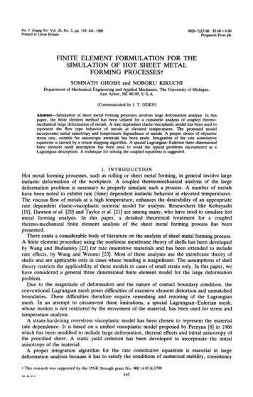
152S. GHOSH and N. KIKUCHIwhere F, G, H, L, M and N are parameters of anisotropy dependent on the state of strain andthe temperature.In eqn (43) directions 1, 2 and 3 correspond to the principal axes ofanisotropy in the unrotated configuration. In sheet metal forming problems we shall assume theprincipal material axes to remain orthogonal in the unrotated configuration, throughout thedeformation process. It is also assumed that the material is transversely isotropic and rotationalisotropy exists in the mid-plane of the sheet metal. Under these assumptions, the effectivestress becomes5’ ; [(F G)t:, (F G)& 2Gt:, - 2Ft11tzz - 2Gt2&- 2Gtll& 2(G 2F)& where {t}’ 6Mt;, 6Mt:,] t [AlW(44) {tllt22t33t12t23t31} andF G-F-G000-FF G-G000-G-G2G0000000000006M0000006k I[A] ;2(G 2F)(45)Purumeters for anisotropy. (a) Initial yield: The parameters of anisotropic yield criterionare determined by tension tests in the 1 and 3 direction and a shear test in the 2-3 plane. Byletting all stresses except the one under consideration to be equal to zero, the initial yieldparameters F,, Go and MO are obtained as:(46)t 30and t230 are the initial yield stresses in the tension and shear in the respectiveho,direction. If the reference direction coincides with the 1 direction, Z. may be chosen to be tloand the parameters will adjust accordingly.(b) Subsequent yield (strain-hardening):The uniaxial static yield stresses for a strainhardening material changes with increasing plastic deformation. The parameters in the effectivestress expression for anisotropic materials are assumed to depend on the plastic work done in astatic process in which rate effects are absent. These parameters represent the work hardeningeffect in a rate independent elastic-plastic process. Their evaluation is based on an assumptionthat for an equivalent change in the effective stress, the plastic work done each direction shouldbe the same. The plastic work may be expressed as:where(47)where a subscript s correspondsmay be written as:to a static condition. The total equivalent plastic rotated strainP (48)

Hot sheet metal forming processesEPEP153&’3311i t211-pE23EPFig. 3. Equating plastic work.Then the parametersare obtained from Fig. 3 as:zG where I,, So, fro, f30 and t230 are the equivalent current maximum stress, the initial equivalentyield stress, the uniaxial initial yield stresses in 1 and 3 directions and the initial yield strengthin shear in the 2-3 plane respectively. The yield strengths correspond to the static yieldcondition. Also Ep, Epl, EP3 and GP are the slopes of the equivalent stress-plastic strain curve,stress-plastic strain in the 1 and 3 directions and the shear stress-plastic shear strain curve in the2-3 plane. The equivalent yield strength may be made to be the same as the yield strengths inany of the directions and the parameters may be adjusted accordingly. The initial yieldstrengths are all temperature dependent.3.2.2. Thermal rate of deformationThe thermal rate of deformationdeformation problems as:followsdirectly0;; cu, bfromthe relationsused for small(50)

S. GHOSH and N. KIKUCHI154where 6 is the rate of temperature change and oij is a temperature dependent coefficient ofthermal expansion. Assuming that aij is a constant isotropic tensor in this analysis, the rotatedrate of thermal deformation becomesd: a S,Swhere 6, is the Kroneckerenergy balance eqn (37).(51)delta, The rate of temperaturechange is obtainedby solving the3.2.3. Visco-plasticrate of deformationThe rate of viscoplastic strain introduced in this section follows from the concept of closestpoint mapping. It is assumed that the onset of viscoplastic behavior is governed by a static yieldcondition and the components of the viscoplastic strain rate tensor are functions of stresses inexcess of the static yield strength. Such a model introduced by Perzyna [S] has been extendedto account for large deformation. The model suffers the disadvantages of not being able toinclude rate dependent initial yield and time dependent strain recovery. Bauschinger effect isalso not included in the model. However, this model has been chosen for the sake of simplicity.A yield function F is used to characterize the material which may be expressed as:F(t, dUp,0) i - K(W , 0)where K is the work hardening parameterThe rotated rate of viscoplastic defo ation(52)with values & for initial yield and 1’,subsequently.tensor may then be written in the formd”J’ y (D(I-K(W‘IP’e)) d”(53)atijwhere y is a temperature dependent viscosity coefficient and ( ) is the MacCauley operator.This model for scoplastic rate of deformation satisfies the in ompressibi ty condition i.e.dz f 0. Normality of this strain rate tensor to the dynamical yield surface (I) in the rotatedstress space is evident from its definition. The function Q (F) may be chosen to take differentforms depending on the material and conditions of the numerical experiment. A form(P(F) Fp has been chosen in the analysis for its proven suitability for metals.In order to have a complete set of rate constitutive relations, it is important to supplementthe stress-strain equation with evolution relations for internal variables. They may be of theform4 f(o, 9)(54)where q are the spatial internal variables and f is a tensor function of stresses and internalvariables. In this analysis the work hardening parameter K has been chosen to be the internalvariable and its rate may be defined as:where 2P is the effective viscopl

metal forming analysis. In this paper, a detailed theoretical treatment for a coupled thermo-mechanical finite element analysis of the sheet metal forming process has been presented. There exists a considerable body of literature on the