WIXLIB

CONTENTS7PrefaceScience has evolved over thousands of years. It began out of curiosity about how the world around us worksas well as a need to know how to make things work better. From water management to space travel, science isessential for success.The evolution of science is layered: Early science depended mostly on critical observation, thus the early scientist was considered a philosopher who created a theory. Soon experiments were designed to test these theories.This process is successful when a new principle is established, leading to a deeper and reproducible experimental observation. This typically takes years. A key component of science is making and testing models, that aredesigned to evaluate the results of experiments quantitatively in a mathematical framework. Good science is observation and experimentation. Great science is the art of making models that explain experimental results. Thisalways results in a deeper question, suggesting new experiments. Each generation has its geniuses. One of thesewas Galileo, who was a philosopher, experimentalist, and mathematician.An understanding of physics requires a knowledge of mathematics. The converse is not true. By definition,pure mathematics contains no physics. Yet historically, mathematics has a rich history filled with physical applications. Mathematics was developed by individuals who intend to make things work. As an engineer, I see thesecreators of early mathematics as budding engineers. This book is an attempt to tell the story of the developmentof mathematical physics as viewed by an engineer.There are two distinct ways to learn mathematics: by learning definitions and relationships, or by associating each mathematical concept with its physical counterpart. Students of physics and engineering best learnmathematics based on the underlying physical concepts. Students of pure mathematics are taught via definitionsof abstract structures, not from the history of mathematical physics. These two teaching methods result in verydifferent understandings of the material.There is a deep common thread between physics and mathematics: the chronological development, or thehistory of mathematics. This is because much of mathematics was developed to solve physical problems. Mostearly mathematics evolved from attempts to understand the world, with the goal of navigating it. Pure mathematicsfollowed as generalizations of these physical concepts.Around 1638 Galileo stated that, based on his experiments with balls rolling down inclined planes and pendulums, the height of a falling object is given byh(t) 1 2Gt ,2(0.0.1)where t is time and G is a constant. This formula leads to a constant acceleration a(t) of the object sincea(t) d2h(t) Gdt2is independent of time. It follows that the force on a body is proportional to its acceleration a, defined as G –namely, F a G. Thus G must be the object’s mass, which must be a constant. If the object has a constantforward velocity, then the object will have a parabolic trajectory. The relative mass may be measured using abalance scale. I believe Galileo understood all this.Years later, following up on the observations from Galileo’s study of pendulums and falling objects, Newtonshowed that differential equations were necessary to explain gravity and that the force of gravity is proportionalto the masses of the two objects divided by the square of the reciprocal of the distance between them:mMd2r(t) G 2 .2dtr (t)To find r(t) we must integrate this equation. For an object at height h(t) above the surface of the earth, r(t) Re h(t) Re , where Re is the radius of earth. In this case, the force is effectively constant, since h Re .Newton’s equation says the acceleration is constant,d2 h(t)mM G 2 ,2dtRe

8CONTENTSbut different from Galileo’s G (a simple mass). Yet it seems clear that the physics behind Newton’s formula forthe acceleration a(t) of two large masses (sun and earth, or earth and moon) and Galileo’s physics for balls rollingdown inclined planes are the same.1 The difference is that Newton’s proportionality constant is a significantgeneralization of Galileo’s. But, other than the constant, which defines the acceleration, the two formulas are thesame.This is not a typical mathematics book; rather, it is about the relationship of math and physics, presentedroughly in chronological order via their history. To teach mathematical physics in an orderly way, our treatmentrequires a step backward in terms of the mathematics, but a step forward in terms of the physics. Historicallyspeaking, mathematics was created by individuals such as Galileo who, by modern standards, may be viewed asengineers. This book contains the basic information that well-informed engineers need to know, as best I canprovide.Let the reader beware that engineering and physics texts do not intend to be rigorous, in the mathematical sense.In some ways, mathematics cleans up the mess by proving theorems, which frequently start with speculations inphysics and even engineering. The cleanup is a slow, tedious process. Just because something seems obviousbased on the known physical facts does not make it a fundamental theorem of mathematics.Although there are similarities between this book and that of Graham et al. (1994), the differences are notable.First, Graham’s Concrete Mathematics presents an impossible standard to be measured against. Second, is isclearly a math book, brilliantly written and targeted at computer science students. This book is not just a mathbook – it is a mathematical physics text, which depends much on underlying math. I would like to believe thereare similarities in (1) the broad range of topics, (2) the in-depth discussion, and (3) the use of historical context.Organization: As discussed in Sec. 1.2.2 and Fig. 1.6 (p. 21), the book is divided into three mathematicalthemes, called streams, presented as five chapters: Introduction, Number Systems, Algebraic Equations, ScalarCalculus, and Vector Calculus. Appendices are used to isolate complex self-contained topics and large tables,such a those for Laplace transforms.Chapter 2, Number Systems, introduces two key concepts, the greatest common divisor (GCD) and the continued fraction algorithm (CFA). When we deal with simple electrical networks composed of inductors, resistors,and capacitors (Fig. 3.8, page 110), or mechanical networks consisting of masses, dashpots, and springs, or theirequivalent, pendulums, as used by Galileo in his studies of gravity (Figs. 1.3, page 16 and 3.11, page 120), thesystem may be modeled as a Brune impedance, defined as the ratio of polynomials of the Laplace frequencys σ ω (see Sec. 3.2.3, page 79 and Sec. 4.4.2, page 144). Of special importance is the development ofordinary differential equations (Sec. 3.4.2, and Eq. 3.4.4) which under generalized symmetry conditions, calledpostulates (Sec. 3.9.1, page 121), characterize Brune impedances (Brune, 1931a).Using the CFA (Sec. 2.5.4), we can generalize the Brune impedance. This generalization results in a transmission line, that describes wave propagation in horns, dealt with in Chapters 4 and 5 (Cauer et al., 1958; Cauer,1958). This topic is both physically and mathematically important (Cauer, 1932).The material is delivered in numbered sections (e.g., Sec. 1.1) spread out over a semester of 15 weeks, threelectures per week, with a three-lecture time-out for administrative duties. Eleven problem sets are provided forweekly assignments.Many students have rated these assignments as the most important part of the course. There is a built-ininterplay between these assignments and the lectures. When a student returns an assignment or exam the fullsolution is provided while it is still fresh in their mind (ateaching moment).Author’s personal statementAn expert is someone who has made all possible mistakes in a small field. I don’t know if I would be called anexpert, but I certainly have made my share of mistakes. I openly state that I love making mistakes because I learnso much from them. One might call that the “expert’s corollary.”This book has been written out of my love for the topic of mathematical physics, a topic that provides manyinsights, that lead to a deep understanding of important physical concepts. Over the years I have developed aphysical sense of math along with a related mathematical sense of physics. While doing my research,2 I believethat math can be physics, and physics math. I have come across what I feel are certain conceptual holes that needfilling, and I sense many deep relationships between math and physics that remain unidentified. What we presentlyteach is not wrong, but it is missing these relationships. What is lacking is an intuition for how math “works.”1 .3.20191002a/full/2 ions

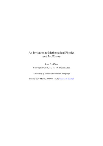
CONTENTS9ENGINEERINGMATHEMATICSPHYSICSFigure 1:There is a natural symbiotic relationship amongmathematics, engineering, and physics (MEP), depicted in theVenn diagram. Mathematics provides the method and rigor. Engineering transforms the method into technology. Physics explores the boundaries. While these three disciplines work welltogether, there is poor communication, in part due to the vastlydifferent vocabularies. But style may be more at issue. Forexample, mathematics rarely uses a system of units, whereasphysics and engineering depend critically on them. Mathematics strives to abstract the ideas into proofs. Physics rarely usesa proof. When they attempt rigor, physicists and engineers typically get into difficulty. An important observation by Felix Kleinabout pure mathematicians, regarding the unavoidable inaccuracies in physics: “It may be said that the idea [of inaccuracy]is usually so repulsive to [mathematicians] that its recognitionsooner or later spoils their interest in natural science” (Condonand Morse, 1929, p. 19).Good scientists “listen” to their data. In the same way, we need to start listening to the language of mathematics.We need to let mathematics guide us toward our engineering goals.As summarized in Fig. 1, this marriage of math, engineering, and physics (MEP)3 helps us make progressin understanding the physical world. We must turn to mathematics and physics when trying to understand theuniverse. My views follow from a lifelong attempt to understand human communication – that is, the perceptionand decoding of human speech sounds. This research arose from my 32 years at Bell Labs in the AcousticsResearch Department. There such lifelong pursuits not only were possible but were openly encouraged. The ideawas that if you are successful at something, take it as far as you can, but, on the other hand, you should not dosomething well that’s not worth doing. People got fired for the latter. I should have left for a university after amere 20 years at Bell Labs,4 but the job was just too cushy.In this text it is my goal to clarify conceptual errors while telling the story of physics and mathematics.My views have been inspired by classic works, as documented in the Bibliography. This book was inspired bymy reading of Stillwell (2002) through his Chapter 21. Somewhere in Chapter 22 I switched to the third edition(Stillwell, 2010), at which point I realized I had much more to master. It became clear that by teaching this materialto first-year engineers, I could absorb the advanced material at a reasonable pace. This book soon followed.SummaryThis is foremost a math book, but not the typical math book. First, this book is for the engineering minded, forthose who need to understand math to do engineering, to learn how things work. In that sense the book is moreabout physics and engineering than mathematics. Math skills are essential for making progress in building things,be it pyramids or computers, as clearly shown by the great civilizations of the Chinese, Egyptians, Mesopotamians,Greeks, and Romans.Second, this is a book about the math that developed to explain physics, to enable people to engineer complexthings. To sail around the world, one needs to know how to navigate. This requires a model of the planets andstars. You can know where you are on earth once you understand where earth is relative to the sun, planets, MilkyWay, and distant stars. The answer to such a cosmic question depends on whom you ask. Who is qualified toanswer such a question? It is best answered by those who study mathematics applied to the physical world. Theutility and accuracy of that answer depend critically on the depth of understanding of the physics of the cosmicclock.The English astronomer Edmond Halley (1656–1742) asked Isaac Newton (1643–1727) for the equation thatdescribes the orbit of the planets. Halley was obviously interested in comets. Newton immediately answered, “anellipse.” It is said that Halley was stunned by the response (Stillwell, 2010, p. 176), as this was what had beenexperimentally observed by Kepler (ca. 1619) and he knew that Newton must have some deeper insight. Bothwere eventually knighted.When Halley asked Newton to explain how he knew, Newton responded, “I calculated it.” But when challengedto show the calculation, Newton was unable to reproduce it. This open challenge eventually led to Newton’s grand3 MEP4Iis a focused alternative to STEM.started around December 1970, fresh out of graduate school, and retired on December 5, 2002.

10CONTENTStreatise, Philosophiae Naturalis Principia Mathematica (July 5, 1687). It had a humble beginning, as a letter toHalley explaining how to calculate the orbits of the planets. To do this Newton needed mathematics, a tool he hadmastered. It is widely accepted that Newton and Gottfried Leibniz invented calculus. But the early record showsthat perhaps Bhaskara II (1114–1185 CE) had mastered the art well before Newton.5Third, the main goal of this book is to teach mathematics to motivated engineers, in a way that it can beunderstood, mastered, and remembered. How can this impossible goal be achieved? The answer is to fill in thegaps with Who did what, and when? Compared with the math, the historical record is easily mastered.To be an expert in a field, one must know its history. This includes who the people were, what they did, and thecredibility of their story. Do you believe the Pope or Galileo on the roles of the sun and the earth? The observablesprovided

An understanding of physics requires a knowledge of mathematics. The converse is not true. By definition, pure mathematics contains no physics. Yet historically, mathematics has a rich history filled with physical appli-cations. Mathematics was developed by individuals who intend to make things work. As an engineer, I see these