WIXLIB

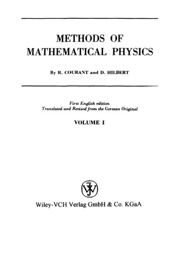
ii“Newman” — 2016/2/8 — 17:00 — page 8 — #24i8i1. Mathematical Preliminarieswhere r̂, θ̂, and ẑ are unit vectors in the associated directions.Similarly, we write the curl of g as gz (r gθ ) gr gz1 r̂ r θ̂ g r θ z z r (r gθ ) gr ẑ . (1.38) r θFinally, the integral over some volume V of a scalar function fcan be written equivalently asVf (x, y, z) dx dy dz VVf (x1 , x2 , x3 ) dx1 dx2 dx3f (x) dV f (x) d3 xVf (r , θ, z)r dr dθ dz.(1.39)VThis concludes our summary of cylindrical coordinates.We now adopt spherical coordinates (Figure 1.1) according tox r sin θ cos ϕy r sin θ sin ϕz r cos θ,(1.40)which can be inverted according to r x 2 y 2 z2 θ arccos(z/r ) arccos z/ x 2 y 2 z2ϕ arctan (y/x).(1.41)Without elaboration, we list here some essential results.1. Unit vector relationships, from which gr , gθ , and gϕ canalso be extracted:r̂ sin θ cos ϕx̂ sin θ sin ϕŷ cos θẑθ̂ cos θ cos ϕx̂ cos θ sin ϕŷ sin θẑϕ̂ sin ϕx̂ cos ϕŷ.(1.42)We note, as a check, that all three of these unit vectors areof unit length and are mutually orthogonal.2. Gradient of a scalar f : f i f1 f1 fr̂ θ̂ ϕ̂. rr θr sin θ ϕ(1.43)i

iii“Newman” — 2016/2/8 — 17:00 — page 9 — #251.2. Cylindrical and Spherical Geometryi9rϕ(x,y,z)θθyϕϕ(x,y,0)rθxFigure 1.1.Spherical coordinates.3. Laplacian of a scalar f : 2 f 1r 2 sin θ f r2 r r f sin θ θ θsin θ 1 2f. (1.44)sin θ ϕ2Note that the Laplacian of vector quantities will differ fromthe above due to the dependence of the projected components on the coordinates.4. Divergence of a vector g: gϕ (r 2 gr ) (sin θgθ )1sin θ r r. ·g 2r sin θ r θ ϕ(1.45)5. Curl of a vector g: (r sin θgϕ ) (r gθ )r̂ ϕ θ (r sin θgϕ ) gr r θ̂ ϕ r (r gθ ) gr r sin θ ϕ̂ . r θ1 g 2r sin θ(1.46)6. Volume integral of a scalar f :Vif (x) d3 x f (r , θ, ϕ)r 2 sin θ dr dθ dϕ.(1.47)Vi

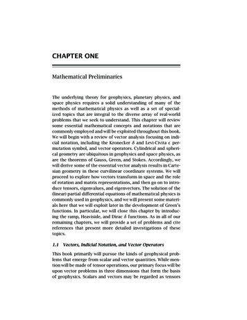
ii“Newman” — 2016/2/8 — 17:00 — page 10 — #26i10i1. Mathematical PreliminariesWe will now review some of the integral relations involving vector quantities.1.3Theorems of Gauss, Green, and StokesWe wish to present some familiar results from integral calculus.We will not provide proofs but will present a brief sketch as tohow they can be obtained. In Figure 1.2, we depict the relevantgeometry.x2Sn̂PCS'Vx1x3Figure 1.2.Geometry of volume and surface.We denote by V the volume under consideration, and S denotesthe surface of that volume. We identify a point P on the surfaceof that volume, and show by an arrow the unit vector n̂ emergingout from that surface. Finally, we draw a closed curve C on thatsurface that contains a surface area S . We denote by g a vector function and by f and h two different scalar functions. Weassume that f , g, and h all go to zero as our distance from theorigin goes to infinity. As before, we denote surface and volumeelements by d2 x and d3 x, respectively.Gauss’s theorem can be expressed byV · g d3 x Sg · n̂ d2 x.(1.48)This result can be proved by subdividing the volume V into a setof cubes, going to the limit that the sides of the cubes becomeii

ii“Newman” — 2016/2/8 — 17:00 — page 11 — #27i1.4. Rotation and Matrix Representationi11vanishingly small. It is simple to show by a direct integrationthat Gauss’s theorem holds for each cube. When we amalgamateall of the cubes, the contributions emerging from the surfacesthat are in common cancel, leaving only the contribution fromthe external enveloping surface.Green’s theorem (Morse and Feshbach, 1999) is generallyexpressed asV · (f h h f ) d3 x S(f h h f ) · n̂ d2 xV(f 2 h h 2 f ) d3 x.(1.49)Other textbooks, for example, Greenberg (1998), refer to this asone of Green’s identities. The second integral is a direct application of Gauss’s theorem. To obtain the third integral, we appliedthe · operator on the product of the two terms and eliminatedthe common f · h term, expressing · as the Laplacian 2 .Stokes’s theorem allows us to relate the integral of the curl ofa vector acting upon the surface S’ that is enclosed by a curve Cto the integral of that vector projected onto and along that curveC. It emerges in electromagnetic theory and has the form 2( g) · n̂ d x g · d ,(1.50) S Cwhere denotes an integral around a closed curve, in this caseC, and d is a differential line element that resides on C. As inthe case of Gauss’s theorem, we can prove Stokes’s theorem bysubdividing the area enclosed by the curve into a set of squareswhose sides will ultimately be taken to be vanishingly small.Stokes’s theorem can readily be proven on a square, and thelines in common among the squares cancel when calculating thecontribution from all squares in the limit.1.4Rotation and Matrix RepresentationWe have already explored one form of vector rotation, namely,the conversion of Cartesian coordinates into spherical geometrywhere the unit vectors x̂, ŷ, and ẑ were replaced by or “rotated”into r̂, θ̂, and ϕ̂. We wish to obtain a general expression for converting coordinates from a system of axes ê1 , ê2 , and ê3 to newcoordinate axes ê1 , ê2 , and ê3 . (We assume that you have had anii

ii“Newman” — 2016/2/8 — 17:00 — page 12 — #28i12i1. Mathematical Preliminariesintroductory linear algebra course as an undergraduate, including the solution of linear equations via Gaussian elimination andintroduction to the eigenvalue problem.) The visual approach tocoordinate conversions as well as rotation is typically presenteddiagrammatically in two dimensions, but becomes rather cumbersome and confusing in three. Matrix algebra provides a simple way of clarifying this problem. We recognize that the newcoordinate axes êi for i 1, 2, 3 should be expressible as a linear combination of the êj coordinate axes. Suppose that A is a3 3 matrix with components Aij so that we can writeêi 3 Aij êj Aij êj(1.51)j 1for i 1, 2, and 3, returning to indicial notation, since this is ageneral expression for a linear combination of the original coordinate axes. Accordingly, we take the dot product of this expression with êk , for i, k 1, . . . , 3 and observe thatêk · êi êi · êk 3 Aij êk · êj Aik(1.52)j 1by virtue of the Kronecker δ identity (1.7). A useful mnemonicdevice for remembering this result is that Aik is the matrix thatconnects the kth axis from the original coordinate to the ith axisin the new coordinate system. Similarly, we introduce anothermatrix B so that we can write the inverse operation, going fromthe new coordinates back to the old, namely,êi 3 Bij êj Bij êj ,(1.53)i 1returning to indicial notation, and directly obtain thatBik êi · êk .(1.54)Bik Aki ,(1.55)We observe thatestablishing that the matrix B Ã where the tilde designatesthe transpose of the matrix. Hence, it immediately follows thatÃA AÃ I,i(1.56)i

iii“Newman” — 2016/2/8 — 17:00 — page 13 — #291.4. Rotation and Matrix Representationi13where I designates the identity matrix so that its ij componentsare δij . For self-evident reasons, we refer to both A and B asrotation matrices.The conversion of the coordinates of a point from one coordinate system to another, which is a rotated version (without translation) of the original, can also be regarded as a rotation in theopposing sense of the point undergoing coordinate conversion.For example, suppose our coordinate conversion correspondedto a positive 45 rotation of the x-y axes to a new x -y set ofaxes, leaving the z-axis unchanged. That would have the sameeffect as a rotation of negative 45 in the x-y plane of the pointunder consideration.Returning momentarily to the expression Aij êi · êj , it follows that each of the matrix components is a direction cosine, theinner product of the original jth unit vector with the new ith unitvector. Had we attempted to do this using a visual construction,for example, as performed by Goldstein et al. (2002), we wouldhave observed the same relationships, albeit in a geometricallycomplicated form. One final feature of rotation matrices that isoften important is that the three rows of a rotation matrix, if wewere to regard them as three vectors, are mutually orthogonaland of unit length. A similar observation can be made for thethree columns of a rotation matrix.Suppose now that we have a vector v that we wish to expressin both coordinate systems utilizing (1.1) and indicial notation,namely,v vi êi v vj êj .(1.57)Taking the inner product of êk with this expression, we observethatvk vj êk · êj êk · êj vj Akj vj .(1.58)Therefore, we note that the Cartesian coordinate representationin the new reference (rotated) frame transforms in the sameway as the coordinate axes transform. For more insight into thenature of rotations, consult Goldstein et al. (2002) or Newman(2012).Before proceeding, it is useful to describe two further aspectsof matrix structure. Any matrix A can be expressed as the sumof a symmetric and an antisymmetric matrix, namely,A iA Ã A Ã ,22(1.59)i

ii“Newman” — 2016/2/8 — 17:00 — page 14 — #30i14i1. Mathematical Preliminarieswhere à designates the transpose of the matrix. Rotation matrices have a special structure, inasmuch as they possess both asymmetric and an antisymmetric part. Intuitively, we expect thata rotation matrix identifies a special direction corresponding tothe axis around which the rotation takes place, and the angleof rotation that is executed around this axis. It takes two variables to identify the direction—think of them as correspondingto a latitude and longitude—and a third variable to identify themagnitude of the rotation. This situation applies whether we areconsidering a physical rotation of an object or the expression ofits orientation in a new coordinate system. Newman (2012) provides a more detailed discussion of this problem. There are othermethodologies for describing a rotation, such as through threeEuler angles. Goldstein et al. (2002) provides a detailed discussion of this approach. The Euler angles are routinely employedin celestial mechanics in describing the orientation of ellipticalorbits in the gravitational two-body problem, for example, forcometary orbits (Roy, 2005).We consider an x-y plane established by the orbit of Jupiteraround the Sun, with the x-direction corresponding to the direction of Jupiter’s perihelion; we wish to establish the orientation of the comet’s elliptical orbit with respect to this invariable plane. To do this, we undertake a series of rotations of thecomet’s orbit. We begin with the ellipse being in the x-y planewith the Sun at the origin, and the ellipse’s axis initially orientedin the x-direction. We then rotate the ellipse in the x-y plane,that is, around the z-axis, by an angle referred to as the longitude of the ascending node Ω. The line of nodes identifies they-axis about which the plane of the orbit is now rotated in thex-z plane to corresponds to its angle of inclination i. Finally,we perform a third rotation, this time around the new z-axisin the x-y plane to identify the longitude of perihelion ω. Fordetails of this procedure, the reader is encouraged to consultGoldstein et al. (2002), Roy (2005), Taff (1985), and Danby (1988).Importantly, what should be evident is that, by executing threesuccessive rotations around the z, y, and z axes, respectively,it is possible to orient properly any three-dimensional object.There are alternative conventions for the Euler angles that aredetailed in Goldstein et al. (2002). We have focused here uponthe one commonly employed in planetary science as well as inii

ii“Newman” — 2016/2/8 — 17:00 — page 15 — #31i1.5. Tensors, Eigenvalues, and Eigenvectorsi15classical mechanics. Rotation matrices occupy an important rolein describing the dynamics of objects and materials in many different environments.A natural question to ask now is, how do matrices derived fromphysically based considerations such as a variational or energyprinciple transform under coordinate axis rotation? This is thedefining characteristic that distinguishes tensors from matrices.1.5Tensors, Eigenvalues, and EigenvectorsIn this section, we will explore how we can make symmetric 3 3matrices transform under coordinate rotation in the same wayas a vector; in so doing, we refer to the matrix as being a secondrank tensor. In addition, we observe that there exists a specialcoordinate basis where the action of the tensor upon a vector isequivalent to a scalar multiplication. This simplifies many calculations, and eigenvalue-eigenvector analysis is at the heart ofthis procedure. We will demonstrate how to solve the eigenvalueproblem, and show how the eigenvectors form the basis set forthe new coordinate system.Having observed (1.57) describing how vectors transform,namely,vi Aij vj B̃ji vj ,(1.60)we introduce the concept of a second-rank tensor T as beinga matrix T with components Tk that transforms similarly,namely, Aik Aj Tk Aik Tk à j B̃ik Tk B jTij(1.61) Bik Tk B̃ j Ãik Tk A j .Tij Bik Bj Tk (1.62)andAccordingly, we writeT AT ÃorT ÃT A,(1.63)which is routinely referred to as a similarity transformation.(Equivalent expressions are available utilizing B.)ii

ii“Newman” — 2016/2/8 — 17:00 — page 16 — #32i16i1. Mathematical PreliminariesMatrix quantities in geophysics are generally real valued andfrequently symmetric; if A is symmetric, we say thatAij Aji .(1.64)Tensors are often associated with situations where there are special associated directions. For example, in geophysics and engineering applications, the stress and strain tensors describe howcompressional or extensional forces act upon materials resulting in a displacement according to a generalization of Hooke’slaw. In particular, if T is a tensor and u is a vector, we can finda number λ such that T · u λu. In this situation, we referto λ as an eigenvalue or characteristic value of T and u is itsassociated eigenvector or characteristic vector . For the examplesmentioned, the stress and strain tensors are symmetric, therebyguaranteeing the existence of real eigenvalues and eigenvectors.Moreover, there are special directions where the force associatedwith a solid or plastic material emerges in a direction orthogonalor normal to a surface (Newman, 2012). Similarly, in rotationalkinematics (see, e.g., Goldstein et al., 2002) the moment of inertiatensor has special directions associated with it, often as an outcome of symmetry considerations. Since most geophysics graduate students have already completed an analytical mechanicscourse, but possibly not continuum mechanics, we shall explorerotational motion as an example of the eigenvalue problem.Suppose we wish to calculate the kinetic energy K of a rigidsolid body rotating around its center of mass with angular velocity ω, where the direction of this vector corresponds to the orientation of the spin axis. It follows, for any point x inside therotating body, that the corresponding velocity isv ω x(1.65)and the kinetic energy satisfies1ρ(x)v 2 (x) d3 x.(1.66)2Importantly, we note that this is an integral over non-negativequantities and must necessarily yield a positive result. Aftersome brief algebra, we find thatK 1ρ(x)[xk xk ωi δij ωj ωi ωj xi xj ] d3 x2 ωi Iij ωj ,K i(1.67)i

iii“Newman” — 2016/2/8 — 17:00 — page 17 — #331.5. Tensors, Eigenvalues, and Eigenvectorsi17which we refer to as a quadratic form where the components ofthe moment of inertia tensor Iij satisfyIij ρ(x)[xk xk δij xi xj ].(1.68)We immediately note that this tensor is real and symmetric.Tensor analysis, especially the properties of eigenvalues andeigenvectors, is an important topic generally treated in advancedundergraduate mathematics courses. However, there are somefeatures of eigenvalue analysis for tensorial quantities that areconceptually vital in geophysics, and we sketch here some oftheir properties. More complete physically motivated treatmentscan be found in Goldstein et al. (2002) and in Newman (2012),which show that 3 3 symmetric tensors have real-valued eigenvalues and eigenvectors. In this particular case, the eigenvaluesmust be positive (or possibly zero) since the kinetic energy cannever be negative. The eigenvalues, in turn, are the solutions tothe cubic (characteristic) polynomial p(λ) constructed by solving for the three roots of the equationp(λ) det(A λI) 0.(1.69)(Please note that we are employing Iij to designate the components of the moment of inertia tensor. Many linear algebra textbooks employ the same symbol to describe the components ofthe identity matrix.) For this physically important class of eigenvalue problems, Cardano’s method (Newman, 2012) provides anexplicit closed-form solution, and we now sketch the derivationof this method.Suppose the cubic polynomial can be expressedaλ3 bλ2 cλ d 0,(1.70)where a 0. We choose to eliminate the quadratic term byreplacing λ with z α, where α b/3a. We now obtain theequationaz3 c z d 0,(1.71)where c c 2αb 3α2 a and d d cα bα2 aα3 . Wenow exploit the triple-angle identitycos3 θ i14cos 3θ 34cos θ,(1.72)i

ii“Newman” — 2016/2/8 — 17:00 — page 18 — #34i18i1. Mathematical Preliminarieswhich can be readily verified by writing cos θ in exponentialform. We replace z in (1.71) by γ cos θ and then obtain aγ 3 cos 3θ3aγ 2 c d 0.(1.73)γ cos θ44We are at liberty to select γ so that the first bracketed term disappears, and we then select θ so that the second bracketed termdisappears. Note, however, that the solution for θ is degenerate; upon finding one solution, we can construct two additionalsolutions that are also real valued by taking our original solution and adding 2π /3 as well as taking our original solutionand subtracting 2π /3. This kind of degeneracy is common incomplex analysis and is associated with branch cuts, a topic wewill review in chapter 3. Remarkably, while often overlooked inmost textbooks, real-world, three-dimensional eigenvalue solutions are readily within reach.Finally, we note that for each of the eigenvalues, we cannow explicitly calculate the eigenvectors by solving the associated pair of linear equations and then normalizing the vectorsobtained to be of unit length. We designate, after ordering, theeigenvalues represented by Ii according to0 I1 I2 I3 .(1.74)(In planetary physics, the eigenvalues are often referred to as0 A B C.) We now define the normalized eigenvectorsassociated with the three eigenvalues as ê , for 1, 2, and 3. Ifthis se

Mathematical Preliminaries The underlying theory for geophysics, planetary physics, and space physics requires a solid understanding of many of the methods of mathematical physics as well as a set of special-ized topics that are integral to the diverse array of real-world problems that we seek to understand. This chapter will review