Transcription
Mathematical Programming:An Overview1Management science is characterized by a scientific approach to managerial decision making. It attemptsto apply mathematical methods and the capabilities of modern computers to the difficult and unstructuredproblems confronting modern managers. It is a young and novel discipline. Although its roots can betraced back to problems posed by early civilizations, it was not until World War II that it became identifiedas a respectable and well defined body of knowledge. Since then, it has grown at an impressive pace,unprecedented for most scientific accomplishments; it is changing our attitudes toward decision-making, andinfiltrating every conceivable area of application, covering a wide variety of business, industrial, military, andpublic-sector problems.Management science has been known by a variety of other names. In the United States, operationsresearch has served as a synonym and it is used widely today, while in Britain operational research seemsto be the more accepted name. Some people tend to identify the scientific approach to managerial problemsolving under such other names as systems analysis, cost–benefit analysis, and cost-effectiveness analysis.We will adhere to management science throughout this book.Mathematical programming, and especially linear programming, is one of the best developed and mostused branches of management science. It concerns the optimum allocation of limited resources amongcompeting activities, under a set of constraints imposed by the nature of the problem being studied. Theseconstraints could reflect financial, technological, marketing, organizational, or many other considerations. Inbroad terms, mathematical programming can be defined as a mathematical representation aimed at programming or planning the best possible allocation of scarce resources. When the mathematical representation useslinear functions exclusively, we have a linear-programming model.In 1947, George B. Dantzig, then part of a research group of the U.S. Air Force known as Project SCOOP(Scientific Computation Of Optimum Programs), developed the simplex method for solving the generallinear-programming problem. The extraordinary computational efficiency and robustness of the simplexmethod, together with the availability of high-speed digital computers, have made linear programming themost powerful optimization method ever designed and the most widely applied in the business environment.Since then, many additional techniques have been developed, which relax the assumptions of the linearprogramming model and broaden the applications of the mathematical-programming approach. It is thisspectrum of techniques and their effective implementation in practice that are considered in this book.1.1AN INTRODUCTION TO MANAGEMENT SCIENCESince mathematical programming is only a tool of the broad discipline known as management science,let us first attempt to understand the management-science approach and identify the role of mathematicalprogramming within that approach.1
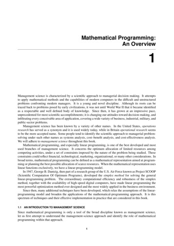
2Mathematical Programming: An Overview1.2It is hard to give a noncontroversial definition of management science. As we have indicated before,this is a rather new field that is renewing itself and changing constantly. It has benefited from contributionsoriginating in the social and natural sciences, econometrics, and mathematics, much of which escape therigidity of a definition. Nonetheless it is possible to provide a general statement about the basic elements ofthe management-science approach.Management science is characterized by the use of mathematical models in providing guidelines tomanagers for making effective decisions within the state of the current information, or in seeking furtherinformation if current knowledge is insufficient to reach a proper decision.There are several elements of this statement that are deserving of emphasis. First, the essence of management science is the model-building approach—that is, an attempt to capture the most significant features of thedecision under consideration by means of a mathematical abstraction. Models are simplified representationsof the real world. In order for models to be useful in supporting management decisions, they have to be simpleto understand and easy to use. At the same time, they have to provide a complete and realistic representationof the decision environment by incorporating all the elements required to characterize the essence of theproblem under study. This is not an easy task but, if done properly, it will supply managers with a formidabletool to be used in complex decision situations.Second, through this model-design effort, management science tries to provide guidelines to managers or,in other words, to increase managers’ understanding of the consequences of their actions. There is never anattempt to replace or substitute for managers, but rather the aim is to support management actions. It is critical,then, to recognize the strong interaction required between managers and models. Models can expedientlyand effectively account for the many interrelationships that might be present among the alternatives beingconsidered, and can explicitly evaluate the economic consequences of the actions available to managers withinthe constraints imposed by the existing resources and the demands placed upon the use of those resources.Managers, on the other hand, should formulate the basic questions to be addressed by the model, and theninterpret the model’s results in light of their own experience and intuition, recognizing the model’s limitations.The complementarity between the superior computational capabilities provided by the model and the higherjudgmental capabilities of the human decision-maker is the key to a successful management-science approach.Finally, it is the complexity of the decision under study, and not the tool being used to investigate thedecision-making process, that should determine the amount of information needed to handle that decisioneffectively. Models have been criticized for creating unreasonable requirements for information. In fact,this is not necessary. Quite to the contrary, models can be constructed within the current state of availableinformation and they can be used to evaluate whether or not it is economically desirable to gather additionalinformation.The subject of proper model design and implementation will be covered in detail in Chapter 5.1.2MODEL CLASSIFICATIONThe management-science literature includes several approaches to classifying models. We will begin with acategorization that identifies broad types of models according to the degree of realism that they achieve inrepresenting a given problem. The model categories can be illustrated as shown in Fig. 1.1.Operational ExerciseThe first model type is an operational exercise. This modeling approach operates directly with the realenvironment in which the decision under study is going to take place. The modeling effort merely involvesdesigning a set of experiments to be conducted in that environment, and measuring and interpreting the resultsof those experiments. Suppose, for instance, that we would like to determine what mix of several crude oilsshould be blended in a given oil refinery to satisfy, in the most effective way, the market requirements forfinal products to be delivered from that refinery. If we were to conduct an operational exercise to support thatdecision, we would try different quantities of several combinations of crude oil types directly in the actual
1.2Model Classification3refinery process, and observe the resulting revenues and costs associated with each alternative mix. Afterperforming quite a few trials, we would begin to develop an understanding of the relationship between theFig. 1.1 Types of model representation.crude oil input and the net revenue obtained from the refinery process, which would guide us in identifyingan appropriate mix.In order for this approach to operate successfully, it is mandatory to design experiments to be conductedcarefully, to evaluate the experimental results in light of errors that can be introduced by measurement inaccuracies, and to draw inferences about the decisions reached, based upon the limited number of observationsperformed. Many statistical and optimization methods can be used to accomplish these tasks properly. Theessence of the operational exercise is an inductive learning process, characteristic of empirical research in thenatural sciences, in which generalizations are drawn from particular observations of a given phenomenon.Operational exercises contain the highest degree of realism of any form of modeling approach, sincehardly any external abstractions or oversimplifications are introduced other than those connected with theinterpretation of the observed results and the generalizations to be drawn from them. However, the methodis exceedingly, usually prohibitively, expensive to implement. Moreover, in most cases it is impossible toexhaustively analyze the alternatives available to the decision-maker. This can lead to severe suboptimizationin the final conclusions. For these reasons, operational exercises seldom are used as a pure form of modelingpractice. It is important to recognize, however, that direct observation of the actual environment underliesmost model conceptualizations and also constitutes one of the most important sources of data. Consequently,even though they may not be used exclusively, operational exercises produce significant contributions to theimprovement of managerial decision-making.GamingThe second type of model in this classification is gaming. In this case, a model is constructed that is anabstract and simplified representation of the real environment. This model provides a responsive mechanismto evaluate the effectiveness of proposed alternatives, which the decision-maker must supply in an organizedand sequential fashion. The model is simply a device that allows the decision-maker to test the performanceof the various alternatives that seem worthwhile to pursue. In addition, in a gaming situation, all the humaninteractions that affect the decision environment are allowed to participate actively by providing the inputsthey usually are responsible for in the actual realization of their activities. If a gaming approach is used in ourprevious example, the refinery process would be represented by a computer or mathematical model, whichcould assume any kind of structure.The model should reflect, with an acceptable degree of accuracy, the relationships between the inputs andoutputs of the refinery process. Subsequently, all the personnel who participate in structuring the decisionprocess in the management of the refinery would be allowed to interact with the model. The production manager would establish production plans, the marketing manager would secure contracts and develop marketing
4Mathematical Programming: An Overview1.2strategies, the purchasing manager would identify prices and sources of crude oil and develop acquisitionprograms, and so forth. As before, several combinations of quantities and types of crude oil would be tried,and the resulting revenues and cost figures derived from the model would be obtained, to guide us in formulating an optimal policy. Certainly, we have lost some degree of realism in our modeling approach withrespect to the operational exercise, since we are operating with an abstract environment, but we have retainedsome of the human interactions of the real process. However, the cost of processing each alternative has beenreduced, and the speed of measuring the performance of each alternative has been increased.Gaming is used mostly as a learning device for developing some appreciation for those complexitiesinherent in a decision-making process. Several management games have been designed to illustrate howmarketing, production, and financial decisions interact in a competitive economy.SimulationSimulation models are similar to gaming models except that all human decision-makers are removed fromthe modeling process. The model provides the means to evaluate the performance of a number of alternatives, supplied externally to the model by the decision-maker, without allowing for human interactions atintermediate stages of the model computation.Like operational exercises and gaming, simulation models neither generate alternatives nor produce anoptimum answer to the decision under study. These types of models are inductive and empirical in nature;they are useful only to assess the performance of alternatives identified previously by the decision-maker.If we were to conduct a simulation model in our refinery example, we would program in advance a largenumber of combinations of quantities and types of crude oil to be used, and we would obtain the net revenuesassociated with each alternative without any external inputs of the decision-makers. Once the model resultswere produced, new runs could be conducted until we felt that we had reached a proper understanding of theproblem on hand.Many simulation models take the form of computer programs, where logical arithmetic operations areperformed in a prearranged sequence. It is not necessary, therefore, to define the problem exclusively inanalytic terms. This provides an added flexibility in model formulation and permits a high degree of realismto be achieved, which is particularly useful when uncertainties are an important aspect of the decision.Analytical ModelFinally, the fourth model category proposed in this framework is the analytical model. In this type of model,the problem is represented completely in mathematical terms, normally by means of a criterion or objective,which we seek to maximize or minimize, subject to a set of mathematical constraints that portray the conditionsunder which the decisions have to be made. The model computes an optimal solution, that is, one that satisfiesall the constraints and gives the best possible value of the objective function.In the refinery example, the use of an analytical model implies setting up as an objective the maximizationof the net revenues obtained from the refinery operation as a function of the types and quantities of the crudeoil used. In addition, the technology of the refinery process, the final product requirements, and the crudeoil availabilities must be represented in mathematical terms to define the constraints of our problem. Thesolution to the model will be the exact amount of each available crude-oil type to be processed that willmaximize the net revenues within the proposed constraint set. Linear programming has been, in the last twodecades, the indisputable analytical model to use for this kind of problem.Analytical models are normally the least expensive and easiest models to develop. However, they introduce the highest degree of simplification in the model representation. As a rule of thumb, it is better to beas much to the right as possible in the model spectrum (no political implication intended!), provided that theresulting degree of realism is appropriate to characterize the decision under study.Most of the work undertaken by management scientists has been oriented toward the development andimplementation of analytical models. As a result of this effort, many different techniques and methodologieshave been proposed to address specific kinds of problems. Table 1.1 presents a classification of the mostimportant types of analytical and simulation models that have been developed.
1.3Formulation of Some Examples5Table 1.1 Classification of Analytical and Simulation ModelsStrategy evaluationStrategy generationCertaintyDeterministic simulationEconometric modelsSystems of simultaneousequationsInput-output modelsLinear programmingNetwork modelsInteger and mixed-integerprogrammingNonlinear programmingControl theoryUncertaintyMonte Carlo simulationEconometric modelsStochastic processesQueueing theoryReliability theoryDecision theoryDynamic programmingInventory theoryStochastic programmingStochastic control theoryStatistics and subjective assessment are used in all models to determine values forparameters of the models and limits on the alternatives.The classification presented in Table 1.1 is not rigid, since strategy evaluation models are used forimproving decisions by trying different alternatives until one is determined that appears ‘‘best.’’ The importantdistinction of the proposed classification is that, for strategy evaluation models, the user must first chooseand construct the alternative and then evaluate it with the aid of the model. For strategy generation models,the alternative is not completely determined by the user; rather, the class of alternatives is determined byestablishing constraints on the decisions, and then an algorithmic procedure is used to automatically generatethe ‘‘best’’ alternative within that class. The horizontal classification should be clear, and is introduced becausethe inclusion of uncertainty (or not) generally makes a substantial difference in the type and complexity ofthe techniques that are employed. Problems involving uncertainty are inherently more difficult to formulatewell and to solve efficiently.This book is devoted to mathematical programming—a part of management science that has a commonbase of theory and a large range of applications. Generally, mathematical programming includes all ofthe topics under the heading of strategy generation except for decision theory and control theory. Thesetwo topics are entire disciplines in themselves, depending essentially on different underlying theories andtechniques. Recently, though, the similarities between mathematical programming and control theory arebecoming better understood, and these disciplines are beginning to merge. In mathematical programming,the main body of material that has been developed, and more especially applied, is under the assumption ofcertainty. Therefore, we concentrate the bulk of our presentation on the topics in the upper righthand cornerof Table 1.1. The critical emphasis in the book is on developing those principles and techniques that leadto good formulations of actual decision problems and solution procedures that are efficient for solving theseformulations.1.3FORMULATION OF SOME EXAMPLESIn order to provide a preliminary understanding of the types of problems to which mathematical programmingcan be applied, and to illustrate the kind of rationale that should be used in formulating linear-programmingproblems, we will present in this section three highly simplified examples and their corresponding linearprogramming formulations.Charging a Blast Furnace An iron foundry has a firm order to produce 1000 pounds of castings containingat least 0.45 percent manganese and between 3.25 percent and 5.50 percent silicon. As these particular castingsare a special order, there are no suitable castings on hand. The castings sell for 0.45 per pound. The foundryhas three types of pig iron available in essentially unlimited amounts, with the following properties: Excel spreadsheet available at http://web.mit.edu/15.053/www/Sect1.3 Blast Furnace.xls
6Mathematical Programming: An Overview1.3Type of pig ironSiliconManganeseAB4 %0.45%1 %0.5%C0.6%0.4%Further, the production process is such that pure manganese can also be added directly to the melt. The costsof the various possible inputs are:Pig APig BPig CManganese 21/thousand pounds 25/thousand pounds 15/thousand pounds 8/pound.It costs 0.5 cents to melt down a pound of pig iron. Out of what inputs should the foundry produce the castingsin order to maximize profits?The first step in formulating a linear program is to define the decision variables of the problem. These arethe elements under the control of the decision-maker, and their values determine the solution of the model.In the present example, these variables are simple to identify, and correspond to the number of pounds of pigA, pig B, pig C, and pure manganeseto be used in the production of castings. Specifically, let us denote thedecision variables as follows:x1 Thousands of pounds of pig iron A,x2 Thousands of pounds of pig iron B,x3 Thousands of pounds of pig iron C,x4 Pounds of pure manganese.The next step to be carried out in the formulation of the problem is to determine the criterion the decisionmaker will use to evaluate alternative solutions to the problem. In mathematical-programming terminology,this is known as the objective function. In our case, we want to maximize the total profit resulting from theproduction of 1000 pounds of castings. Since we are producing exactly 1000 pounds of castings, the totalincome will be the selling price per pound times 1000 pounds. That is:Total income 0.45 1000 450.To determine the total cost incurred in the production of the alloy, we should add the melting cost of 0.005/pound to the corresponding cost of each type of pig iron used. Thus, the relevant unit cost of the pigiron, in dollars per thousand pounds, is:Pig iron APig iron BPig iron C21 5 26,25 5 30,15 5 20.Therefore, the total cost becomes:Total cost 26x1 30x2 20x3 8x4 ,(1)and the total profit we want to maximize is determined by the expression:Total profit Total income Total cost.Thus,Total profit 450 26x1 30x2 20x3 8x4 .(2)
1.3Formulation of Some Examples7It is worthwhile noticing in this example that, since the amount of castings to be produced was fixed inadvance, equal to 1000 pounds, the maximization of the total profit, given by Eq. (2), becomes completelyequivalent to the minimization of the total cost, given by Eq. (1).We should now define the constraints of the problem, which are the restrictions imposed upon the valuesof the decision variables by the characteristics of the problem under study. First, since the producer does notwant to keep any supply of the castings on hand, we should make the total amount to be produced exactlyequal to 1000 pounds; that is,1000x1 1000x2 1000x3 x4 1000.(3)Next, the castings should contain at least 0.45 percent manganese, or 4.5 pounds in the 1000 pounds ofcastings to be produced. This restriction can be expressed as follows:4.5x1 5.0x2 4.0x3 x4 4.5.(4)The term 4.5x1 is the pounds of manganese contributed by pig iron A since each 1000 pounds of this pig ironcontains 4.5 pounds of manganese. The x2 , x3 , and x4 terms account for the manganese contributed by pigiron B, by pig iron C, and by the addition of pure manganese.Similarly, the restriction regarding the silicon content can be represented by the following inequalities:40x1 10x2 6x3 32.5,40x1 10x2 6x3 55.0.(5)(6)Constraint (5) establishes that the minimum silicon content in the castings is 3.25 percent, while constraint(6) indicates that the maximum silicon allowed is 5.5 percent.Finally, we have the obvious nonnegativity constraints:x1 0,x2 0,x3 0,x4 0.If we choose to minimize the total cost given by Eq. (1), the resulting linear programming problem canbe expressed as follows:Minimize z 26x1 30x2 20x3 8x4 ,subject to:1000x14.5x140x140x1 1000x2 1000x3 5.0x2 4.0x3 10x2 6x3 10x2 6x3x1 0,x2 0,x3 0,x4 1000,x4 4.5, 32.5, 55.0,x4 0.Often, this algebraic formulation is represented in tableau form as follows:Total lbs.ManganeseSilicon lowerSilicon upperObjective(Optimal solution)Decision variablesx1x2x3x41000 1000 100014.554140106040106026302080.77900.220 0.111Relation Requirements10004.532.555.0z (min)25.54The bottom line of the tableau specifies the optimal solution to this problem. The solution includesthe values of the decision variables as well as the minimum cost attained, 25.54 per thousand pounds; thissolution was generated using a commercially available linear-programming computer system. The underlyingsolution procedure, known as the simplex method, will be explained in Chapter 2.
8Mathematical Programming: An Overview1.3Fig. 1.2 Optimal cost of castings as a function of the cost of pure manganese.It might be interesting to see how the solution and the optimal value of the objective function is affectedby changes in the cost of manganese. In Fig. 1.2 we give the optimal value of the objective function as thiscost is varied. Note that if the cost of manganese rises above 9.86/lb., then no pure manganese is used. In therange from 0.019/lb. to 9.86 lb., the values of the decision variables remain unchanged. When manganesebecomes extremely inexpensive, less than 0.019/lb., a great deal of manganese is used, in conjuction withonly one type of pig iron.Similar analyses can be performed to investigate the behavior of the solution as other parameters of theproblem (for example, minimum allowed silicon content) are varied. These results, known as parametricanalysis, are reported routinely by commercial linear-programming computer systems. In Chapter 3 we willshow how to conduct such analyses in a comprehensive way.Portfolio Selection A portfolio manager in charge of a bank portfolio has 10 million to invest. Thesecurities available for purchase, as well as their respective quality ratings, maturities, and yields, are shownin Table 1.2.Table overnmentMunicipalQuality scalesMoody’sAaAaAaaAaaBaBank’s22115Years tomaturity915432Yield 2.24.5The bank places the following policy limitations on the portfolio manager’s actions:1. Government and agency bonds must total at least 4 million.2. The average quality of the portfolio cannot exceed 1.4 on the bank’s quality scale. (Note that a lownumber on this scale means a high-quality bond.)3. The average years to maturity of the portfolio must not exceed 5 years.Assuming that the objective of the portfolio manager is to maximize after-tax earnings and that the tax rate is50 percent, what bonds should he purchase? If it became possible to borrow up to 1 million at 5.5 percent Excel spreadsheet available at http://web.mit.edu/15.053/www/Sect1.3 Portfolio Selection.xls
1.3Formulation of Some Examples9before taxes, how should his selection be changed?Leaving the question of borrowed funds aside for the moment, the decision variables for this problem aresimply the dollar amount of each security to be purchased:xAxBxCxDxE Amount to be invested in bond A; in millions of dollars. Amount to be invested in bond B; in millions of dollars. Amount to be invested in bond C; in millions of dollars. Amount to be invested in bond D; in millions of dollars. Amount to be invested in bond E; in millions of dollars.We must now determine the form of the objective function. Assuming that all securities are purchased at par(face value) and held to maturity and that the income on municipal bonds is tax-exempt, the after-tax earningsare given by:z 0.043xA 0.027xB 0.025xC 0.022xD 0.045xE .Now let us consider each of the restrictions of the problem. The portfolio manager has only a total of tenmillion dollars to invest, and therefore:xA xB xC xD xE 10.Further, of this amount at least 4 million must be invested in government and agency bonds. Hence,xB xC xD 4.The average quality of the portfolio, which is given by the ratio of the total quality to the total value of theportfolio, must not exceed 1.4:2xA 2xB xC xD 5xE 1.4.xA xB xC xD xENote that the inequality is less-than-or-equal-to, since a low number on the bank’s quality scale means ahigh-quality bond. By clearing the denominator and re-arranging terms, we find that this inequality is clearlyequivalent to the linear constraint:0.6xA 0.6xB 0.4xC 0.4xD 3.6xE 0.The constraint on the average maturity of the portfolio is a similar ratio. The average maturity must notexceed five years:9xA 15xB 4xC 3xD 2xE 5,xA xB xC xD xEwhich is equivalent to the linear constraint:4xA 10xB xC 2xD 3xE 0.Note that the two ratio constraints are, in fact, nonlinear constraints, which would require sophisticatedcomputational procedures if included in this form. However, simply multiplying both sides of each ratioconstraint by its denominator (which must be nonnegative since it is the sum of nonnegative variables)transforms this nonlinear constraint into a simple linear constraint. We can summarize our formulation intableau form, as follows:xAxBCash11Governments1Quality0.6 0.6Maturity410Objective0.043 0.027(Optimal solution) 3.36 0xC11 0.4 10.0250xD11 0.4 20.0226.48xE1Relation Limits 10 43.6 0 3 00.045 z (max)0.160.294
10Mathematical Programming: An Overview1.3The values of the decision variables and the optimal value of the objective function are again given in the lastrow of the tableau.Now consider the additional possibility of being able to borrow up to 1 million at 5.5 percent beforetaxes. Essentially, we can increase our cash supply above ten million by borrowing at an after-tax rate of 2.75percent. We can define a new decision variable as follows:y amount borrowed in millions of dollars.There is an upper bound on the amount of funds that can be borrowed, and hencey 1.The cash constraint is then modified to reflect that the total amount purchased must be less than or equal tothe cash that can be made available including borrowing:xA xB xC xD xE 10 y.Now, since the borrowed money costs 2.75 percent after taxes, the new after-tax earnings are:z 0.043xA 0.027xB 0.025xC 0.022xD 0.045xE 0.0275y.We summarize the formulation when borrowing is allowed and give the solution in tableau form as ective(Optimal solution)xA1xB1xC1xD1xE10.640.0433.7010.6100.02701 0.4 10.02501 0.4 20.0227.133.6 30.0450.18y 11 0.02751Relation Limits101400z (max)0.296Production and Assembly A division of a plastics company manufactures three basic products: sporks,packets, and school packs. A spork is a plastic utensil which purports to
1.1 AN INTRODUCTION TO MANAGEMENT SCIENCE Since mathematical programming is only a tool of the broad discipline known as management science, let us first attempt to understand the management-science approach and identify the role of mathematical programming within that approach. 1