Transcription
MATHEMATICAL MODELING USING R PROGRAMMINGENVIRONMENT – SOME EXAMPLESLeslie ChandrakanthaJohn Jay College of Criminal Justice of CUNYMathematics and Computer Science Department524 West 59th Street, New York, NY 10019lchandra@jjay.cuny.eduAbstractIn this paper, we explain how to use simulation to study mathematical modeling. Thesimulations are performed using the R programming environment. We use two examplesto demonstrate the modeling activities. For each case, the description of the model,simulation steps, and the solution are discussed. R codes for each case are also provided.IntroductionA mathematical model is a description of a real situation using mathematical concepts.The process of creating a mathematical model for a given problem is called mathematicalmodeling. Many mathematical models relate to real life problems and that areinterdisciplinary in nature. Blomhoj and Jensen [5] have given the following six steps toformulate and solve problems using mathematical modeling. These include: formulation,selection of relevant objects and relations, translation of these objects and relation tomathematics, use of mathematical methods to obtain the results, interpretation of theresults to make conclusions, and evaluation of the validity of the models. Students oftenfail to connect and apply what they have learnt in introductory mathematics courses toother subjects, sometimes leading to the belief that mathematics is not relevant to them.Due to this lack of problem solving skills, teaching mathematical modeling is achallenging task to many instructors [14]. Sometimes due to the unpredictable andunexpected outcomes of mathematical modeling tasks, instructors may be discouraged tointroduce modeling activities in the classroom [4].Technology and technology based environment will allow instructors and students toalleviate these shortcomings and lack of problem solving skills in mathematical modeling[1]. Technology should not replace the entire modeling process, but only providetemporary means to overcome the difficulties. The approaches of teaching mathematicalmodeling have been influenced by the development and introduction of technologies suchas graphing calculators and computer software [10]. Many researchers have reported the
successful use of technology in introducing mathematical ideas. For instance, the use of aspreadsheet to explore mathematical concepts has been discussed by Chua and Wu [7] fora secondary classroom, and by Beare [3] at college level. Ang and Awyong [2] reportedthat the use of computer algebra systems such as Maple in some tertiary courses has beenwell received. Not surprisingly, the use of technology continues to prevail in themathematics classroom at all levels. The acquisition of the knowledge of the technologieswill be an essential part before applying them in mathematical modeling. We believe theuse of technology continues to prevail in the mathematics classroom at all levels.In this paper, we describe how to use R with some programming or coding capabilities insolving mathematical models. We use a simulation approach to find the solutions. R isincreasingly being used as a tool for mathematical and statistical education. Manymathematics instructors use R to teach and perform calculations. Although it is bitchallenging to write statements in the command line, R can be used in simulationeffectively. A valuable introduction to R for introductory courses is given in [12]. We usetwo examples to demonstrate mathematical modeling and solving. In coming section, wegive introduction to simulation modeling, a brief overview of R, and modeling andsolving two examples. We end with some concluding remarks.Simulation ModelingA simulation model is a mathematical model, which combines both mathematical andlogical concepts that try to imitate the operations of a real life process or system throughuse of computer software. The computer simulation approach has been used inmathematical modeling and solving complex problems [13]. In recent times, manyinstructors use simulation in their classroom to explain the difficult concepts [6]. Incertain situations, relevant data are not readily available or cannot be obtained. In thesesituations, simulation modeling provides ways to study such problems.In the simulation process, a computer program or a software application is used togenerate steps that are formulated to model and solve the given problem. Based on theassumptions and the rules of the problem, outcomes or the values of the variables of themodel are calculated iteratively until desired results are obtained. There are manytechnological tools and computer programming languages available to perform suchsimulations. In this paper, we use R for this process. R is freely available to instructorsand students.Brief Overview of RR is a free software environment used for working with data. R can be used to createsophisticated graphs, carry out statistical analyses, and run simulations. It is also aprogramming language with a set of built-in-functions. With some knowledge of coding,
students can write their own codes for mathematical and statistical computations. Forcomputationally intensive tasks, one can incorporate functions written in otherslanguages such as C, C , and FORTRAN. R compiles and runs on Windows, MacOS,and a wide variety of UNIX platforms. The examples of R used in this paper come fromthe most recent version of R, R 3.4.0. R is available from http://www.r-project.org. Toinstall R 3.4.0 on your operating system, download R from the site above using theclosest mirror site to your location and choose the appropriate link for your operatingsystem.R is a relatively simple syntax-driven and case-sensitive language. Even though thesyntax for writing instructions may be somewhat difficult initially, most students withlittle or no prior programming experience have become comfortable using R. In thisparticular course about 50% of the students are Computer Information Systems majorsand they have taken at least one computer programming course prior to taking thiscourse. The other 50% are from quantitative disciplines such as sciences and economics,and have been exposed to some sort of computer logic. R is installed into the schoolcomputers, located in the computer labs which also serve as the location for this course.R is an object-oriented program that works with data structures such as vectors (onedimensional array) and data frames (two dimensional arrays). A vector contains a list ofvalues. When R is started, we will see a window that is called the R console. This iswhere we type our commands and see the text results. Graphics appear in a separatewindow. The is called the prompt, where R commands are written. To quit R we type q( ).R can be used as a calculator. At the prompt, we enter the mathematical expression andby hitting ―enter‖, it will calculate the result and display it. The standard arithmeticoperators ‗ , -, *,‘ and ‗/‘ are used in expressions and ‗ ‘ is used for exponentiation. Thefollowing example demonstrates this: 2*3 -10[1] -4The results of a calculation can be assigned to a variable (object in R) using - or . Inthis paper, we will use -. Even though we can work with single numbers (scalars), R isprimarily designed to work with vectors and functions. In R, a vector is a sequence ofdata values of the same type. The function, c, is used to create vectors from scalars. Thefollowing statement creates a vector: x - c(2, 4, 6, 8, 10) x[1] 2 4 6 8 10Once we have a vector of numbers, we can apply built-in functions to get usefulstatistical summaries and visual displays. R also provides functions for generatingrandom samples from various probability distributions.
Random Numbers using sample functionThe sample function in R generates a sample of specified size from a set of values usingwith or without replacement. Let‘s suppose values are stored in a vector named x. Totake a random sample of size n without replacement from the set x, we use following Rcommand: sample(x, n)To obtain a sample of size n with replacement, we use following command sample(x, n, replace TRUE)We can use the sample function to obtain a random number from a set of numbers, say 1through 10, in following way: sample(1:10,1)[1] 2Control StructuresR has the standard control structures such as if, while, and for, which can be used tocontrol the flow of an R code. We will demonstrate the use of control structures in Rusing the following code segment. Let‘s assume that we have stored 1000 numbers in thevector named x. The following code will compute the average of the nonnegativenumbers in vector x. The symbol # is used to write comments. sum - 0# variable sum initialized to 0 count - 0# variable count initialized to 0 for(i in 1:1000){ if (x[i] 0) { count - count 1# count the positive values sum - sum x[i] }# add the positive values } average - sum/count# compute the averageIn the above code segment, the for loop iterates 1000 times, selecting only nonnegativenumbers using the if statement. It computes the average as well. The variable namedcount counts the number of nonnegative numbers stored in x. We will use the controlstructures when we discuss simulations in the following sections.
ExamplesIn this section, we illustrate two examples that use simulation modeling. All thesimulations are performed using R. For each case, we provide the R code that performsthe simulations.Example One: Chaos GameWe consider a game called the ―chaos game‖. The game is played as follows. First pickthree points and draw a triangle. It can be any triangle. Label the vertices as A, B, and C.Start with any point, say P, inside the triangle. Next take a three sided die with side 1,side 2, and side 3, and roll. There will be three possible outcomes (side 1, 2, or 3) withequal probability. Then continue the game based on the each of the possible outcomesgiven below: If the die rolled side 1, find the midpoint between P and A.If the die rolled side 2, find the midpoint between P and B.If the die rolled side 3, find the midpoint between P and C.Use this midpoint and repeat this process to get next point and continue this process toget the subsequent points. Figure 1 shows the results of simulation of this game with 10rolls of the die. We want to find what will happen if we repeat this process a largenumber of times.Figure 1: Results of 10 rolls of the game
The following R code simulates this process 10,000 times. plot(0:2,0:2,type "n") x - c(0,1,2) y - c(0,2,0) points(x,y,pch 19) labels - c("A","B","C") text(x .05,y,labels) segments(0,0,2,0) segments(0,0,1,2) segments(1,2,2,0) points(1,1,pch 19) X - c() Y - c() X[1] - 1 Y[1] - 1 for(i in 2:10000){ r - sample(1:3,1) if (r 1){ X[i] - (X[i-1] 0)/2 Y[i] - (Y[i-1] 0)/2} else if (r 2){ X[i] - (X[i-1] 1)/2 Y[i] - (Y[i-1] 2)/2} else { X[i] - (X[i-1] 2)/2 Y[i] - (Y[i-1] 0)/2} points(X[i],Y[i],pch 19)}In beginning of the code, plot function with type ―n‖ provides a 2 by 2 empty plot. Thepoints function with pch 19 plots three solid points (0, 0), (1, 2), and (2,0). The textfunction labels those points A, B, and C. The segments function connects the threevertices of the triangle. Then the game starts with a point inside the triangle. In this case,we start at the point (1, 1) using points(1,1, pch 19). Then we create X and Y vectors tohold the points created inside the triangle in each iteration of the simulation. The for loopgenerates and plots 9,999 points (first of 10,000 points is created before for loop begins)inside the triangle. The sample function simulates the rolling the die by generating arandom integer number from 1 to 3. Figure 2 shows the results of simulating the game10,000 times.
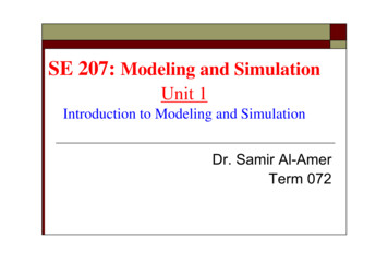
Figure 2: Results of simulating 10,000 timesThe goal of the chaos game is to roll the die many times and predict what the resultingpattern of points will be. Most students who are unfamiliar with the game guess that theresulting image will be a random smear of points. Others predict that the points willeventually fill the entire triangle. The resulting image is anything but a random smear thatthe points form what mathematicians call the Sierpinski triangle [8] shown in abovefigure. Even though this example does not involve a real life problem, it illustrates theuse of simulation for problem solving. It is impossible to predict the outcome or theemerging pattern of this game without simulation process.Example Two: Secretary ProblemThe Secretary problem is also known as the best choice problem that has been examinedextensively in mathematics [11]. Imagine an administrator wanting to hire a secretaryfrom n applicants with the following conditions: n applicants are ranked from best to worst without ties.The applicants are interviewed one by one in random order.The decision about each applicant is to be made immediately after the interview.Once rejected, an applicant cannot be recalled.During the interview, the administrator can rank the applicant among allapplicants interviewed so far, but is unaware of the quality of yet unseenapplicants.We propose the following strategy that will maximize the probability of choosing the bestapplicant from the set of n applicants. Selecting the first applicant is not a wise strategybecause the first applicant has no one to be compared with. Since the decision must bemade immediately after interviewing an applicant, if we wait until last applicant is
interviewed, we may miss out earlier better applicants. A reasonable strategy is to rejecta certain number of applicants, say k-1 of the n applicants, and then choose the firstapplicant that is better than all the previous applicants. If no such applicant exists, thenwe accept the last applicant. Figure 3 illustrates this strategy.Figure 3: Illustration of rejecting first k-1 applicants and selecting next best oneAccording to this strategy, the probability of selecting the best applicant is always at least1/e (about 37%) (see [9] for details]. It further suggests that always rejecting thefirst n/e applicants that are interviewed (e is the base of the natural logarithm and has thevalue 2.71828) and then stopping at the first applicant who is better than every applicantinterviewed so far (or continuing to the last applicant if this never occurs). This strategyselects the best applicant about 37% of times.Now we show how to use R to simulate this process with the above strategy and tocompute the success rate (or empirical probability) of selecting best applicant. As anexample, we take ten applicants (n 10) and assume that we reject the first 3 (k-1 3)applicants before we consider the rest of them. In each iteration of the simulationprocess, we randomly rank 10 applicants from 1 to 10. The following R code simulatesthe process 10 times and finds the selected applicant for each iteration. count - 0 for (i in 1:10){ x - sample(1:10,10) cat("Applicants' Rank: ", x, "\n") y - c() y[1] - y[2] - y[3] - 0 for (j in 4:9){ if (max(x[1:j-1]) x[j] && max(y[1:j-1]) 0) y[j] - x[j] else y[j] - 0} if (max(y[4:9]) 0){ y[10] - x[10]} else { y[10] - 0}
for (j in 4:10){ if (y[j] ! 0) select - j} cat("Selected Applicant: ", select, "\n") if (max(x[1:10]) max(y[4:10])) count - count 1}The output of the above code for first three iterations given below:Applicants' Rank: 10 8 5 4 3 9 2 7 6 1Selected Applicant: 10Applicants' Rank: 6 3 4 2 1 8 7 9 10 5Selected Applicant: 6Applicants' Rank: 9 4 5 7 8 1 10 3 6 2Selected Applicant: 7In the above R code, the variable count is initialized to zero and it counts the number oftimes the best applicant is selected in the simulation process. Then the for loop is used torepeat the simulation 10 times. The sample function generates 10 random digits from 1 to10 randomly without replacement. These 10 numbers are the ranks of the ten applicants.These ranks are displayed using the cat function. Then a y vector is created and assigns 0or the rank of the selected applicant. Since first three applicants are not selected, y[1],y[2], and y[3] get zeros. Among the rest of the applicants, an applicant is selected if theapplicant‘s rank is better than the previous applicants. Then the value of y for thatapplicant is the corresponding value of x, and others get 0. If there is no such applicant,last applicant in the list gets selected. The last if statement counts the number of times thebest applicant is selected.We have simulated this process 10,000 times and counted the number of times the bestapplicant is selected. Dividing this count by 10,000 gives the proportion of times the bestapplicant is selected in this strategy. Our simulation process gave this proportion as0.3964. This means our simulation model approximates the best solution to 39.6%. Thisis close to the 37% that is given in the literature of this problem.ConclusionWe have demonstrated how to use R to model and solve two examples in mathematicalmodeling. This simulation approach is useful in the classroom to model and visualize thesolutions for situations when it is difficult to construct the real physical experiment. Thekey concern is that the students need to have a basic understanding of computer codingand logical thinking to be successful in this approach. In many quantitative disciplines,
students take at least one course in basic computer programming. Therefore students whowant to learn mathematical modeling using technology would not have much difficulty tosucceed using this approach.References[1] Ang, K. C. (2010) Teaching and learning mathematical modeling with technology.Proceedings of the 15th Asian Technology Conference in Mathematics, Kuala Lumpur,Malaysia, 19-29.[2] Ang, K. C., & Awyong, P. W. (1999). The Use of Maple in First Year UndergraduateMathematics. The Mathematics Educator, 4(1), 87-96.[3] Beare, R. (1996). Mathematical Modelling Using a New Spreadsheet-based System,Teaching Mathematics and Its Applications, 15(1), 120-128.[4] Blum, W. & Niss, M. (1991). Applied mathematical problem solving, modelling,applications, and links to other subjects — State, trends and issues in mathematicsinstruction. Educational Studies in Mathematics, 22(1), 37-68.[5] Blomhoj, M. and Jensen, T. H. (2003). Developing mathematical modelingcompetence: Conceptual clarification and educational planning. Teaching Mathematicsand its Applications, 22, 123-139.[6] Chandrakantha, Leslie. (2014), Visualizing and Understanding Confidence Intervalsand Hypothesis Testing Using Excel Simulation. The Electronic Journal ofMathematics and Technology (EJMT), 8(3), 212-221.[7] Chua, B. & Wu, Y. (2005). Designing Technology-Based Mathematics Lessons:A Pedagogical Framework. Journal of Computers in Mathematics and ScienceTeaching, 24(4), 387-402.[8] Devaney, R. (2004). Chaos Rules!, Math Horizon, November , 11-14.[9] Ferguson, T. S., (1989). Who solved the Secretary Problem? Statistical Sciences,4(3), 282-296.[10] Ferrucci, B.J. & Carter, J.A. (2003). Technology-active mathematical modeling,International Journal of Mathematical Education in Science and Technology, 34(5),663-670.[11] Freeman, P.R. (1983).The Secretary Problem and Its Extensions: A Review,International Statistical Review, 51(2), 189-206.[12] James, G, Witten, D, Hastie, T, & Tishirani, R. (2013). An Introduction toStatistical Learning with Applications in R, Springer, New York.[13] Veltern, Kai. (2009). Mathematical Modeling and Simulation, Introduction toScientist and Engineers, WILEY, New York.
[14] Wedelin, D., Adawi, T., Jahan, T., & Anderson, S. (2013). Teaching and learningmathematical modeling and problem solving: A case study. International Conference ofthe Portuguese Society for Engineering Education (CISPEE) , 1 – 6.
The process of creating a mathematical model for a given problem is called mathematical modeling. Many mathematical models relate to real life problems and that are interdisciplinary in nature. Blomhoj and Jensen [5] have given the following six steps to formulate and solve problems using mathematical modeling. These include: formulation,