Transcription
Gaussian Process-Based PredictiveModeling for Bus RidershipSourav BhattacharyaHelsinki Institute forInformation Technology HIITDepartment of ComputerScienceUniversity of Helsinki, Finlandsourav.bhattacharya@cs.helsinki.fiArto KlamiHelsinki Institute forInformation Technology HIITDepartment of ComputerScienceUniversity of Helsinki, Finlandarto.klami@cs.helsinki.fiSanti PhithakkitnukoonComputing DepartmentThe Open University, UKsanti.phi@open.ac.ukMarco VelosoCentro de Informática eSistemasUniversidade de Coimbra,Portugalmveloso@dei.uc.ptPetteri NurmiHelsinki Institute forInformation Technology HIITDepartment of ComputerScienceUniversity of Helsinki, Finlandpetteri.nurmi@cs.helsinki.fiCarlos BentoCentro de Informática eSistemasUniversidade de Coimbra,Portugalbento@dei.uc.ptAbstractThe dynamics of a city are characterized, among others,by the traveling patterns of its dwellers. Accurateknowledge of human mobility patterns would haveapplications, e.g., in urban design, in the optimization ofpublic transportation operating costs, and in theimprovement of public transportation services. Thepresent paper combines a large scale bus transportationdataset with publicly available data sources to predict bususage. We propose a Gaussian process-based approach formodeling and predicting bus ridership. To validate ourapproach we perform experiments on data collected fromLisbon, Portugal. The results demonstrate significantimprovements in prediction accuracy compared to aprobabilistic baseline predictor.Author KeywordsGaussian process, modeling and urban computing.ACM Classification KeywordsTheory of computation [Machine learning approaches]:Gaussian processes.IntroductionCopyright is held by the author/owner(s).UbiComp ’13 Adjunct, Sept 8-12, 2013, Zurich, Switzerland.ACM 978-1-4503-2139-6/13/09. 15.00.It is well known that optimized public transit can reducecongestion, gasoline consumption, and overall carbonfootprint [5, 13]. From a customer perspective, however, a
mobility choice is only a choice if it is fast, comfortable,and reliable. Therefore, strategies for increasing publictransit ridership and improving user satisfaction are anactive and ongoing area of research.Transit authorities are increasingly taking advantage ofpervasive sensing technologies to provide new types ofintelligent transportation services and to understandtransit usage. As an example, services that enabletravelers to access real-time transit vehicle location,arrival time, connection, and other related pieces ofinformation are emerging (e.g., [6, 8, 17]). From a publictransport management perspective, this real-timeinformation can help to improve service and resourcemanagement effectiveness, and hence also ridership anduser satisfaction.The present paper investigates how the combination ofdata collected from pervasive sensors (ticketing and busarrival information) and public, open data sources(weather and transit network information) can be used toenhance public transportation systems, e.g., for serviceand resource management such as dispatching andscheduling. Specifically, we propose a Gaussianprocess-based technique for modeling and predicting busridership, i.e., the number of passengers using a specificbus stop at a given period of time. The proposed modelallows efficient estimation of the ridership rates in variouscontexts. Besides modeling the weekly and dailyfluctuations in bus usage, the model allows incorporatingadditional predictors, such as the weather conditions ordemographic information.Most of present day public transport systems, such asbuses, are operating with fixed schedules, respectively forweekdays, weekends, night hours, and holidays. Makinguse of historical logs and contextual information, such asweather and time contexts, can give more insights intothe dynamics of ridership demands and user behavior,paving way towards adaptive public transport systems thatare responsive to user need and demands. This approachalso contributes to the visions of adaptive transportationsystems [3, 4] and the ’swam’ concept introduced in the2006 UK Government’s Foresight program (i.e.,on-demand public transport systems).We validate our approach using data collected fromLisbon, Portugal, demonstrating that our GaussianProcess-based predictor achieves significantly betterperformance than a probabilistic baseline predictor.Related WorkThe idea of using pervasive sensing in traffic engineeringwas first introduced by Zito et al. [18] who investigatedthe use of GPS for intelligent highway services. Recentadvances in information and communication technologieshave led to development of several services for transportsystems. Camacho et al. [2] presented an overview ofIT-based services offered in public transport, anddiscussed how passenger-centric services can improvepublic transport systems, particularly service quality andpassenger satisfaction.Availability of public transportation data such as train andbus arrival times opens up new directions for researchersto get a better understanding of the current systems andseek ways to improve upon them. Ferrari et al. [7]described a methodology for measuring accessibility ofpublic transportation system-based on analysis ofunderground train data, whereas Patnaik et al. [10]developed a predictive model for bus arrival times. Pinelet al. [11] presented a method to measure accessibility ofa city using bus probe data. Uno et al. [15] proposed a
Data DescriptionWe consider a dataset containing bus informationcollected over a period of two months (April-May 2010)by one of the largest bus operators in Lisbon, Portugal.The dataset consists of two parts: 1) bus probe data and2) ticketing data. The bus probe data contains arrivalinformation of buses at various stops along theirpredefined route. The ticketing data, on the other hand,contains information about passengers getting on a bus.Below we describe the datasets in greater detail andinclude description of publicly available weather data andapplied data pre-processing.Bus Probe DataThe bus probe dataset contains information of bus arrivaltimes at 2, 104 bus stops along various bus routes in thecity of Lisbon. Overall, the dataset containsmeasurements from 96 different bus lines comprising of187 bus routes1 . During the period of two months, over650, 000 bus trips were recorded. The mobility context ofa bus was captured by recording bus ID,heading/direction, bus stop ID, arrival time at a bus stopand bus stop location (latitude, longitude). The locationsof the bus stops considered in this study are shown in1 Bus routes are calculated by considering different directions ofjourney by a bus-line, e.g., ’Up’, ’Down’ or ’Circular’Figure 1 overlaid on the road network of Lisbon (courtesyof OpenStreetMap2 ).Ticketing DataThe second part of the dataset contains bus ridershipinformation collected during passenger ticketing. Nearlyall bus riders in Lisbon use a transit pass, which is apre-purchased card that allows the user to use a busservice. When the user uses the transit pass to enter thebus, the card ID is recorded along with a timestamp andbus specific information such as vehicle ID and bus routeID. During the study period of two months, 812, 170anonymized unique passengers were recorded in theticketing data.38.7838.76Latitudemethodology to evaluate road network-based on traveltime stability and reliability using bus probe data. Bejanet al. [1] developed a model for bus journey timeestimation and examined influential factors such as timeof the day and day of the week. Sun et al. [14] analyzedencounter patterns of people using bus GPS and ticketingdata and found regularity in the patterns, which wasshown as an empirical evidence of the ’familiar strangers’concept in social network tudeFigure 1: Spatial distribution of all bus stops on top of theroad network in the city of Lisbon, Portugal.Weather dataWe augment the Lisbon transportation data with weatherinformation, e.g., temperature, humidity, rain and thunder2 http://www.openstreetmap.org/
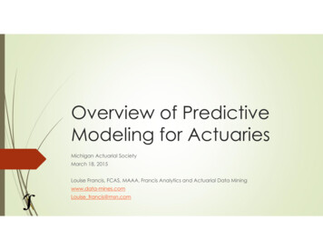
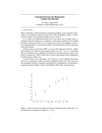
extracted from a publicly available weather data source(courtesy of Weather Underground3 ) that providesweather indicators every half an hour.Data Pre-processingBefore analysis, we process the dataset by removing allbus lines that are not present in both datasets. The busprobe and ticketing datasets were collected independently,but can be combined to generate ridership information bymatching all passengers’ boarding times recorded in theticketing dataset to a specific bus arrival time present inthe bus probe dataset. More specifically, given theboarding time of a passenger and the bus line ID, wesearch all records of the same bus line for the day andidentify the passenger’s bus stop as the one havingsmallest positive time difference to the arrival times of abus at various stops along the bus route.The resultingintegrated data is shown in Figure 2, which shows theridership per hour recorded at two bus stops for a periodof one week. The plot indicates a clear difference in busridership during weekdays and weekends, additionally itclearly shows the existence of a daily cycle.Modeling Bus RidershipFor predicting the number of people getting on a bus webuild separate predictive models for each of the bus stops.The task then is to create a model that takes as input aset of variables describing the current context and providesas an output the expected number of passengers enteringa bus in that context. In the simplest case, the context isdefined as the time of day and the day of week, but in themore general case the context variables should provide allthe information that is needed for making the prediction,such as the weather conditions or the demographics of thedestinations that can be reached by the busline.3 http://www.wunderground.com/In the present work we first introduce models that usetime as the only context. In particular, we model the dailyand hourly fluctuations, depicted in Figure 2, bydescribing the context with two variables: the day of theweek d and the time of the day h (discretized intoone-hour intervals). The task then is to estimate7 24 168 parameters µd,h that describe the expectednumber of passengers getting on a bus at that given time.We propose using Gaussian process (GP) regression [12]for solving the problem, but also present a baseline modelthat simply counts the passengers in the training data forcomparative analysis.After addressing the task of modeling the weekly andhourly cycles in passenger volume, we demonstrate howthe proposed GP model directly extends to richer contextsthat enable more accurate predictions. In particular, weincorporate the current weather conditions into the model.Baseline AlgorithmTo model the passenger counts we define µd,h as theexpected number of passengers getting on any bus thatarrives at the stop during day d and hour h. Given areasonably large collection of training data, we candirectly estimate these parameters as the average numberof passengers seen entering in that temporal context. Weuse ptd,h to denote the number of passengers using thestop during day d and hour h for a given training index(week) t, and ntd,h to denote the number of buses usingthe stop. Then the expected number of passengersentering a bus at those conditions can be estimated as:PTtt 1 pd,hµd,h PT,(1)tt 1 nd,hwhere T denotes the number of weeks present in thetraining data. Besides intuitive reasoning, the model can
Passengers seen60MON50TUEWEDTHUBus-stop 194Bus-stop 0612180612180612180Figure 2: Variation of number of passengers using two bus stops recorded over a period of one week.be justified as the maximum likelihood estimator forobservations that are assumed to follow a normaldistribution. For predicting the ridership for a future testcase, we simply multiply the expected count with theobserved number of buses:p̂d,h nd,h · µd,h .(2)This baseline model makes reasonably accuratepredictions in well-defined discrete contexts. It effectivelyjust looks at the history and predicts that the number ofpassengers will equal that of the mean count in thehistory, which is often a reasonable prediction. Even amodel with T 1 which just predicts that the number ofpassengers will be the same as it was during the sametime last week is useful; we will later demonstrate this asthe comparison model. However, the model breaks downif we attempt to extend it to richer contexts. It estimatesthe ratio separately for each possible context, and henceneeds discrete context variables. The richer the context,the more parameters are needed in the model and, morecrucially, the more training data is needed to accuratelyestimate the parameters. It cannot make reasonablepredictions for contexts that did not occur in the trainingdata, and for rich context this will necessarily be the casefor several if not majority of the contexts.Gaussian Process ModelAs described above, the straightforward approach oflooking back at historical data cannot work for richcontexts. Instead, we need to learn models that generalizeover nearby contexts. Even if the training data had noexamples of the passenger count at Wednesday 3PMwhen it is raining, the model should provide a reasonableestimate by borrowing information about rainy afternoonsin other days and the usual count of passengers nearWednesday 3PM. This task can in general be solved bylearning the parameters for different contexts together andby regularizing the solutions towards each other.In this article we propose to solve the contextual ridershipproblem by a nonparametric Bayesian approach calledGaussian process regression [12], a powerful probabilisticinference technique that has gained popularity in recentyears. It is a regression technique that predicts µ, theexpected number of passengers, for arbitrary contextsusing a nonlinear mapping from the context variables tothe output while constraining the predictions of similar
contexts to be close. The GP regression model isnonparametric, which means that we do not need tospecify the functional form of the mapping in advance,and in particular need not restrict to modeling the outputswith any simple family such as linear functions. Instead,we only need to define a way of computing similaritybetween the contexts in the form of a kernel function.The kernel function then implicitly defines a family ofsmooth functions between the contexts and the outputs.We denote the context by x, which is a vector over thecontext variables, for example x [h, d] in the case oftemporal context only. The output variable in the trainingdata is computed as y pd,h /nd,h . The GP regressionmodel then specifies that the independent variable y arenoisy versions of an arbitrary non-linear function f (x),where f (x) has a Gaussian process prior. This prior,which is on the functions themselves, specifies that thejoint distribution of f (x) and f (x0 ) for any x and x0 isGaussian, and that the covariance of these two is given bya similarity kernel k(x, x0 ). This similarity kernel uniquelydefines the properties of the GP prior space.The actual model is defined asy f , φ Πni 1 p(yi fi , φ),(3)f (x θ) GP(m(x), k(x, x0 )),(4)p(θ)p(φ),(5)θ, φ where the observations y [yi , . . . , yn ]T are assumed tobe conditionally independent given the function valuesf (x), GP(m(x), k(x, x0 )) is the GP prior, and θ and φare hyperparameters of the likelihood and kernel functionswith some suitable prior distributions. To fully specify themodel we need to fix the likelihood function, the kernelfunction, and the prior distributions for thehyperparameters.We start with the likelihood, choosing the Studentt-distribution given by:y f , ν, σs Πni 1Γ((ν 1)/2) Γ(ν/2) νπσs (yi fi )21 νσs2 (ν 1)/2,where ν is the degrees of freedom and σs is the scale ofthe observation noise, dictating how close to the functionvalues f ( x) the observations are likely to fall. We chosethe t-distribution instead of the computationally easiernormal distribution due to its robustness to outliers [9],which might be prevalent in our data especially forlow-volume stops; even if the average rate is very low, aparty of several people might occasionally get on a bus,creating a strong outlier.The choice of the kernel function determines how thefunctions f (x) behave in the space of all possiblecontexts, controlling the smoothness of the predictions.We adopt the common choice of Gaussian kernel function0k(x, x ) σa2Pdexp( k 1 (xk 2lk2x0k )2),(6)where σa2 controls the amplitude of the functions and thelk parameters are the length-scales for individual contextvariables. We could also use other kernels to encodedifferent kind of relationships between the contexts, butthe Gaussian kernel is a flexible choice for modelingcontinuous and ordinal context parameters.Learning the GP model consists of specifying the valuesfor the hyperparameters, in our case φ (ν, σs ) for thelikelihood function and θ (σa , {lk }dk 1 ) for the kernelfunction. The values for these parameters uniquely definethe predictions of the model, and hence there is no needto learn anything else; the model has no actual
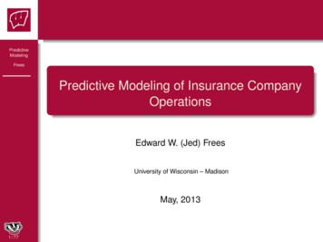
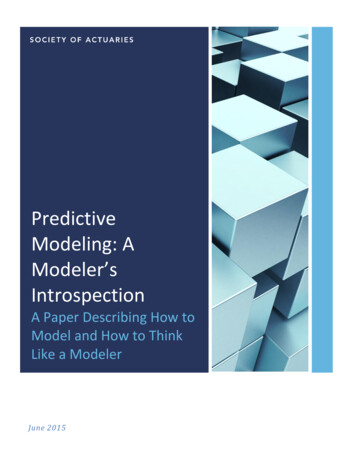
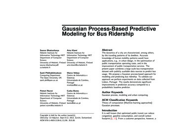
parameters for the mappings themselves, but instead itdefines the predictions indirectly as the posteriordistribution of the function values f (x) for unseen testcontexts. The most important hyperparameters are thelength scales lk , which control the smoothness of thepredictions; the larger lk is for a specific context variablethe smoother the predictions are because of borrowinginformation from a broader range along that variable.For learning the parameters we use Bayesian inference,namely the Markov chain Monte Carlo (MCMC)technique. Instead of learning specific values for theparameters, we compute the predictions by integratingover the posterior distribution of the hyperparametervalues, using the GPstuff package [16] and the defaultchoices for the prior parameters as provided in thepackage. These predictions cannot be expressed in closeform analytical solution, but they are computationallyefficient for reasonably sized training collections. That is,for any given context x observed at the test time we cancompute the expected count µ. Furthermore, we directlyget confidence intervals for the predictions.Figure 3: Scatter plot ofobserved bus ridership with itsprediction obtained from GPmodel.ResultsTo illustrate the proposed modeling framework, weconduct a number of experiments on the Lisbontransportation dataset. After the pre-processing and dataintegration we split the data into individual weeks andperformed a 5-fold cross validation to illustrate thepredictions and to compare the GP model with thebaseline. We always train the models with one week oftraining data and apply it for predicting the passengercount for the remaining weeks, separately for each of thebus stops. To measure the quality of the prediction we useroot mean-square error (RMSE) measure.We start with the simple temporal context of the day ofweek and the hour of day, learning both the GP modeland the baseline model. Figure 3 shows the crossplot ofthe observed counts and the predictions made by the GPmodel, showing that the model does reasonably well. Itsomewhat overestimates the highest counts and thepredictions are noisy, but the correlation between thepredictions and the true values is high (R 0.93). Thecorresponding plot for the baseline model would besimilar, but noisier.To compare the two models in quantitative terms, wecompute the RMSE for each of the bus stops, resulting inan average error of 5.1 for GP and 5.7 for the baselinemodel. A McNemar test indicated that the resultingdifference is statistically significant (p 0.01.) Figure 4illustrates the difference by plotting the cumulativeaverage RMSE over all the bus stops.As an exemplary illustration of GP model, we choose onebus stop and plot the bus ridership for ’Wednesday’ inFigure 6. The plot includes the mean prediction and theconfidence intervals provided by the MCMC integration.The actual observations covering 8 weeks of test datatypically fall within the confidence bounds. Figure 5 showsthe posterior distribution of the length scale parameter lkfor the variable h. The mode of the distribution is around3, indicating that the learned kernel for the hourinfluences the bus ridership prediction significantly for aduration of 3 neighboring hours.Finally, to illustrate the way the GP model can handlericher contexts, we apply the model on data that include abinary indicator telling whether it rains or
9GP ModelAvg. Model860Mean predictionTrue Bus RidershipConfidence Interval503530Bus 15002000501234Length-scale5Figure 5: Histogram of thesampled length-scale parameterfor the hour variable obtainedduring MCMC sampling.6Figure 4: Cumulative RMSE over all bus stops with a 5-foldcross validation.not. We train the model using one week of data, chosenso that there is instances of rain during the week, andthen apply it on the remaining weeks. This results insmall improvement, i.e., average RMSE from 4.95 to 4.93,in the prediction accuracy (with p 0.02 i.e., significantat the 95% level).Conclusion and Future WorkIdentifying factors influencing bus ridership is animportant step, both towards understanding the dynamicsof a city and towards enabling on-demand intelligenttransportation services. In this work we proposed aGaussian process-based predictive model that usescontexts, e.g., time day of the week, hour and raininformation to predict bus ridership. We evaluated ourapproach using two months of bus data collected fromLisbon, Portugal. The GP model results in accurate busridership predictions even with a small amount of trainingdata, and is capable of generalizing across contexts.00510Hours of operation1520Figure 6: Illustration of the GP prediction for ’Wednesday’ atone of the stops. The observed test samples fall usually withinthe confidence interval, and the mean prediction closelyapproximates them.Through experimental analysis we showed that theperformance of GP outperforms a simple probabilisticbaseline. By complementing the temporal context with asimple weather indicator, we also demonstrated that richercontextual descriptions can further improve predictiveaccuracy. Even though the improvement in accuracy wasonly marginal, the experiment acts as a proof of conceptthat the modeling framework can be extended to includemore complex contexts, e.g., temperature, demographicinformation, bus line popularity, proximity to touristicattraction, etc. We plan to include rich context modelingusing GP as our future work.AcknowledgementS. Bhattacharya has received funding from the FutureInternet Graduate School (FIGS) and the Foundation ofNokia Corporation. A. Klami and P. Nurmi acknowledgeTEKES (Tivit Data to Intelligence program) for funding.
References[1] Bejan, A., Gibbens, R., Evans, D., Beresford, A.,Bacon, J., and Friday, A. Statistical modelling andanalysis of sparse bus probe data in urban areas. In13th IEEE Intelligent Transportation SystemsConference, IEEE (September 2010).[2] Camacho, T., Foth, M., and Rakotonirainy, A.Pervasive technology and public transport :opportunities beyond telematics. IEEE PervasiveComputing 12, 1 (2013), 18–25.[3] Cervero, R., and Beutler, J. Adaptive transit:Enhancing suburban transit services. University ofcalifornia transportation center, working papers,University of California Transportation Center, 2000.[4] Crainic, T. G., Errico, F., Malucelli, F., and Nonato,M. Designing the master schedule fordemand-adaptive transit systems. Annals OR 194, 1(2012), 151–166.[5] Davis, T., and Hale, M. Public transportation’scontribution to u.s. greenhouse gas reduction. Tech.rep., 2007.[6] Dziekan, K., and Kottenhoff, K. Dynamic at-stopreal-time information displays for public transport:effects on customers. Transportation Research PartA: Policy and Practice 41 (2007), 489–501.[7] Ferrari, L., Berlingerio, M., Calabrese, F., andCurtis-Davidson, B. Measuring public-transportaccessibility using pervasive mobility data. IEEEPervasive Computing 12, 1 (2013), 26–33.[8] Ferris, B., Watkins, K., and Borning, A. Onebusaway:A transit traveller information system, 2010.[9] Jylänki, P., Vanhatalo, J., and Vehtari, A. Robustgaussian process regression with a student-tlikelihood. J. Mach. Learn. Res. 12 (Nov. 2011),3227–3257.[10] Patnaik, J., Chien, S., and Bladikas, A. Estimationof bus arrival times using apc data. Journal of PublicTransportation 7, 1 (2004), 1–20.[11] Pinel, F., Hou, A., Calabrese, F., Nanni, M., Zegras,C., and Ratti, C. Space and time-dependant busaccessibility: A case study in rome. In 12th IEEEIntelligent Transportation Systems Conference, IEEE(September 2009), 1–6.[12] Rasmussen, C. E., and Williams, C. K. I. Gaussianprocesses for machine learning. The MIT Press, 2006.[13] Schrank, D., and Lomax, T. Urban mobility reporttexas transportation institute. Tech. rep., 2009.[14] Sun, L., Axhausen, K., Lee, D.-H., and Huang, X.Understanding metropolitan collective encounterpatterns. arXiv 1301, 5979 (January 2013).[15] Uno, N., Kurauchi, F., Tamura, H., and Iida, Y.Using bus probe data for analysis of travel timevariability. Journal of Intelligent TransportationSystems: Technology, Planning, and Operations 13,1 (2009), 2–15.[16] Vanhatalo, J., Riihimaki, J., Hartikainen, J., Jylanki,P., Tolvanen, V., and Vehtari, A. Bayesian modelingwith gaussian processes using the gpstuff toolbox,2013. http://mloss.org/software/view/451/.[17] Zimmerman, J., Tomasic, A., Garrod, C., Yoo, D.,Hiruncharoenvate, C., Aziz, R., Thiruvengadam,N. R., Huang, Y., and Steinfeld, A. Field trial oftiramisu: crowd-sourcing bus arrival times to spurco-design. In Proceedings of the SIGCHI Conferenceon Human Factors in Computing Systems, CHI ’11,ACM (New York, NY, USA, 2011), 1677–1686.[18] Zito, R., D’Este, G., and Taylor, M. Globalpositioning systems in the time domain: How usefula tool for intelligent vehicle-highway systems?Transportation Research C 3, 4 (1995), 193–2009.
Modeling Bus Ridership For predicting the number of people getting on a bus we build separate predictive models for each of the bus stops. The task then is to create a model that takes as input a set of variables describing the current context and provides as an output the expected number of passengers entering a bus in that context.