WIXLIB

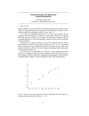
Gaussian Processes for Regression:A Quick IntroductionM. Ebden, August 2008Comments to mark.ebden@eng.ox.ac.uk1M OTIVATIONFigure 1 illustrates a typical example of a prediction problem: given some noisy observations of a dependent variable at certain values of the independent variable , what isour best estimate of the dependent variable at a new value, ?If we expect the underlying functionto be linear, and can make some assumptions about the input data, we might use a least-squares method to fit a straightline (linear regression). Moreover, if we suspectmay also be quadratic, cubic, oreven nonpolynomial, we can use the principles of model selection to choose among thevarious possibilities.Gaussian process regression (GPR) is an even finer approach than this. Ratherthan claimingrelates to some specific models (e.g.), a Gaussianprocess can representobliquely, but rigorously, by letting the data ‘speak’ moreclearly for themselves. GPR is still a form of supervised learning, but the training dataare harnessed in a subtler way.As such, GPR is a less ‘parametric’ tool. However, it’s not completely free-form,and if we’re unwilling to make even basic assumptions about, then more general techniques should be considered, including those underpinned by the principle ofmaximum entropy; Chapter 6 of Sivia and Skilling (2006) offers an introduction.1.510.5?y0 0.5 1 1.5 2 2.5 1.6 1.4 1.2 1 0.8 0.6 0.4 0.200.2xFigure 1: Given six noisy data points (error bars are indicated with vertical lines), weare interested in estimating a seventh at.1

2D EFINITION OF A G AUSSIAN P ROCESSGaussian processes (GPs) extend multivariate Gaussian distributions to infinite dimensionality. Formally, a Gaussian process generates data located throughout some domainsuch that any finite subset of the range follows a multivariate Gaussian distribution.Now, the observations in an arbitrary data set,, can always beimagined as a single point sampled from some multivariate ( -variate) Gaussian distribution, after enough thought. Hence, working backwards, this data set can be partneredwith a GP. Thus GPs are as universal as they are simple.Very often, it’s assumed that the mean of this partner GP is zero everywhere. Whatrelates one observation to another in such cases is just the covariance function,.A popular choice is the ‘squared exponential’,(1)where the maximum allowable covariance is defined as— this should be high forfunctions which cover a broad range on the axis. If, thenapproachesthis maximum, meaningis nearly perfectly correlated with. This is good:for our function to look smooth, neighbours must be alike. Now if is distant from, we have instead, i.e. the two points cannot ‘see’ each other. So, forexample, during interpolation at new values, distant observations will have negligibleeffect. How much effect this separation has will depend on the length parameter, , sothere is much flexibility built into (1).Not quite enough flexibility though: the data are often noisy as well, from measurement errors and so on. Each observation can be thought of as related to an underlyingfunctionthrough a Gaussian noise model:(2)something which should look familiar to those who’ve done regression before. Regression is the search for. Purely for simplicity of exposition in the next page, wetake the novel approach of folding the noise into, by writing(3)whereis the Kronecker delta function. (When most people use Gaussianprocesses, they keepseparate from. However, our redefinition ofis equally suitable for working with problems of the sort posed in Figure 1. So, givenobservations , our objective is to predict , not the ‘actual’ ; their expected valuesare identical according to (2), but their variances differ owing to the observational noiseprocess. e.g. in Figure 1, the expected value of , and of , is the dot at .)To prepare for GPR, we calculate the covariance function, (3), among all possiblecombinations of these points, summarizing our findings in three matrices:.(4)(5)Confirm for yourself that the diagonal elements of are, and that its extremeoff-diagonal elements tend to zero when spans a large enough domain.2

3H OW TO R EGRESS USING G AUSSIAN P ROCESSESSince the key assumption in GP modelling is that our data can be represented as asample from a multivariate Gaussian distribution, we have that(6)where indicates matrix transposition. We are of course interested in the conditionalprobability: “given the data, how likely is a certain prediction for ?”. Asexplained more slowly in the Appendix, the probability follows a Gaussian distribution:(7)Our best estimate foris the mean of this distribution:(8)and the uncertainty in our estimate is captured in its variance:(9)We’re now ready to tackle the data in Figure 1.1. There areobservations , atWe knowfrom the error bars. With judicious choices ofand (moreon this later), we have enough to calculate a covariance matrix using (4):From (5) we also have2. From (8) and (9),andand.3. Figure 1 shows a data point with a question mark underneath, representing theestimation of the dependent variable at.We can repeat the above procedure for various other points spread over some portionof the axis, as shown in Figure 2. (In fact, equivalently, we could avoid the repetitionby performing the above procedure once with suitably largerandmatrices.In this case, since there are 1,000 test points spread over the axis,would beof size 1,000 1,000.) Rather than plotting simple error bars, we’ve decided to plot, giving a 95% confidence interval.3

1.510.5y0 0.5 1 1.5 2 2.5 1.6 1.4 1.2 1 0.8 0.6 0.4 0.200.2xFigure 2: The solid line indicates an estimation of95% confidence intervals are shaded.4for 1,000 values of. PointwiseGPR IN THE R EAL WORLDThe reliability of our regression is dependent on how well we select the covariancefunction. Clearly if its parameters — call them— are not chosen sensibly, the result is nonsense. Our maximum a posteriori estimate of occurswhenis at its greatest. Bayes’ theorem tells us that, assuming we have littleprior knowledge about what should be, this corresponds to maximizing,given by(10)Simply run your favourite multivariate optimization algorithm (e.g. conjugate gradients, Nelder-Mead simplex, etc.) on this equation and you’ve found a pretty goodchoice for ; in our example,and.It’s only “pretty good” because, of course, Thomas Bayes is rolling in his grave.Why commend just one answer for , when you can integrate everything over the manydifferent possible choices for ? Chapter 5 of Rasmussen and Williams (2006) presentsthe equations necessary in this case.Finally, if you feel you’ve grasped the toy problem in Figure 2, the next two examples handle more complicated cases. Figure 3(a), in addition to a long-term downwardtrend, has some fluctuations, so we might use a more sophisticated covariance function:(11)The first term takes into account the small vicissitudes of the dependent variable, andthe second term has a longer length parameter () to represent its long-term4

(b)(a)5643421yy200 1 2 2 3 4 4 1012345 56x 10123x4567Figure 3: Estimation of (solid line) for a function with (a) short-term and long-termdynamics, and (b) long-term dynamics and a periodic element. Observations are shownas crosses.trend. Covariance functions can be grown in this way ad infinitum, to suit the complexity of your particular data.The function looks as if it might contain a periodic element, but it’s difficult to besure. Let’s consider another function, which we’re told has a periodic element. Thesolid line in Figure 3(b) was regressed with the following covariance function:(12)The first term represents the hill-like trend over the long term, and the second termgives periodicity with frequency . This is the first time we’ve encountered a casewhere and can be distant and yet still ‘see’ each other (that is,for).What if the dependent variable has other dynamics which, a priori, you expect toappear? There’s no limit to how complicatedcan be, provided is positivedefinite. Chapter 4 of Rasmussen and Williams (2006) offers a good outline of therange of covariance functions you should keep in your toolkit.“Hang on a minute,” you ask, “isn’t choosing a covariance function from a toolkita lot like choosing a model type, such as linear versus cubic — which we discussedat the outset?” Well, there are indeed similarities. In fact, there is no way to performregression without imposing at least a modicum of structure on the data set; such is thenature of generative modelling. However, it’s worth repeating that Gaussian processesdo allow the data to speak very clearly. For example, there exists excellent theoretical justification for the use of (1) in many settings (Rasmussen and Williams (2006),Section 4.3). You will still want to investigate carefully which covariance functionsare appropriate for your data set. Essentially, choosing among alternative functions isa way of reflecting various forms of prior knowledge about the physical process underinvestigation.5

5D ISCUSSIONWe’ve presented a brief outline of the mathematics of GPR, but practical implementation of the above ideas requires the solution of a few algorithmic hurdles as opposedto those of data analysis. If you aren’t a good computer programmer, then the codefor Figures 1 and 2 is at /GPtut.zip,and more general code can be found at http://www.gaussianprocess.org/gpml.We’ve merely scratched the surface of a powerful technique (MacKay, 1998). First,although the focus has been on one-dimensional inputs, it’s simple to accept those ofhigher dimension. Whereas would then change from a scalar to a vector,would remain a scalar and so the maths overall would be virtually unchanged. Second,the zero vector representing the mean of the multivariate Gaussian distribution in (6)can be replaced with functions of . Third, in addition to their use in regression, GPsare applicable to integration, global optimization, mixture-of-experts models, unsupervised learning models, and more — see Chapter 9 of Rasmussen and Williams (2006).The next tutorial will focus on their use in classification.R EFERENCESMacKay, D. (1998). In C.M. Bishop (Ed.), Neural networks and machine learning.(NATO ASI Series, Series F, Computer and Systems Sciences, Vol. 168, pp. 133166.) Dordrecht: Kluwer Academic Press.Rasmussen, C. and C. Williams (2006). Gaussian Processes for Machine Learning.MIT Press.Sivia, D. and J. Skilling (2006). Data Analysis: A Bayesian Tutorial (second ed.).Oxford Science Publications.A PPENDIXImagine a data sample taken from some multivariate Gaussian distribution with zeromean and a covariance given by matrix . Now decompose arbitrarily into twoconsecutive subvectors and — in other words, writingwould be thesame as writing(13)where , , and are the corresponding bits and pieces that make up .Interestingly, the conditional distribution of given is itself Gaussian-distributed.If the covariance matrixwere diagonal or even block diagonal, then knowingwouldn’t tell us anything about : specifically,. On the other hand, ifwere nonzero, then some matrix algebra leads us to(14)The mean,, is known as the ‘matrix of regression coefficients’, and the variance,, is the ‘Schur complement of in ’.In summary, if we know some of , we can use that to inform our estimate of whatthe rest of might be, thanks to the revealing off-diagonal elements of .6