Transcription
The Gaussian or Normal PDF, Page 1The Gaussian or Normal Probability Density FunctionAuthor: John M. Cimbala, Penn State UniversityLatest revision: 11 September 2013The Gaussian or Normal Probability Density Function Gaussian or normal PDF – The Gaussian probability density function (also called the normal probabilitydensity function or simply the normal PDF) is the vertically normalized PDF that is produced from asignal or measurement that has purely random errors.2 x x 2 1122 .e exp o The normal probability density function is f x 2 2 2 2 o Here are some of the properties of this special distribution: It is symmetric about the mean.f(x) The mean and median are both equal to ,Small the expected value (at the peak of thedistribution). [The mode is undefined for asmooth, continuous distribution.] Its plot is commonly called a “bell curve”because of its shape.Large The actual shape depends on the magnitudeof the standard deviation. Namely, if issmall, the bell will be tall and skinny, whilex if is large, the bell will be short and fat, assketched. Standard normal density function – All of the Gaussian PDF cases, for any mean value and for any standarddeviation, can be collapsed into one normalized curve called the standard normal density function.o This normalization is accomplished through the variable transformations introduced previously, i.e.,x z and f z f x , which yields f z f x oo1e z2/2 1exp z 2 / 2 .2 2 This standard normal density function is valid forany signal measurement, with any mean, and withany standard deviation, provided that the errors(deviations) are purely random.A plot of the standard normal (Gaussian) densityfunction was generated in Excel, using the aboveequation for f(z). It is shown to the right.It turns out that the probability that variable x liesbetween some range x1 and x2 is the same as theprobability that the transformed variable z liesbetween the corresponding range z1 and z2, wherez is the transformed variable defined above. In other words,x x P x1 x x2 P z1 z z2 where z1 1and z2 2. ooo Note that z is dimensionless, so there are no units to worry about, so long as the mean and the standarddeviation are expressed in the same units.x2z2Furthermore, since P x1 x x2 f x dx , it follows that P x1 x x2 z f z dz .x11We define A(z) as the area under the curve between 0 and z, i.e., the special case where z1 0 in theabove integral, and z2 is simply z. In other words, A(z) is the probability that a measurement lieszbetween 0 and z, or A z 0 f z dz , as illustrated on the graph below.
The Gaussian or Normal PDF, Page 2ooFor convenience, integral A(z) is tabulated in statistics books, but it can be easily calculated to avoid theround-off error associated with looking up and interpolating values in a table.1 z f(z)A(z)Mathematically, it can be shown that A z erf 2 2 where erf( ) is the error function, defined as2 2erf exp d . 0zoz0Below is a table of A(z), produced using Excel, which hasa built-in error function, ERF(value). Excel has anotherfunction that can be used to calculate A(z), namely A z NORMSDIST ABS( z) 0.5 .oTo read the value of A(z) at a particular value of z, Go down to the row representing the first two digits of z. Go across to the column representing the third digit of z. Read the value of A(z) from the table. Example: At z 2.54, A(z) A(2.5 0.04) 0.49446. These values are highlighted in the abovetable as an example. Since the normal PDF is symmetric, A( z) A(z), so there is no need to tabulate negative values of z.
The Gaussian or Normal PDF, Page 3 Linear interpolation:o By now in your academic career, you should be able to linearlyzA(z)interpolate from tables like the above.2.540.49446o As a quick example, let’s estimate A(z) at z 2.546.o The simplest way to interpolate, which works for both increasing and2.546A(z) ?decreasing values, is to always work from top to bottom, equating the2.550.49461fractional values of the known and desired variables.o We zoom in on the appropriate region of the table, straddling the z value of interest, and set up forinterpolation – see sketch. The ratio of the red difference to the blue difference is the same for eitherA z 0.494612.546 2.55 column. Thus, keeping the color code, we set up our equation as.2.54 2.55 0.49446 0.494612.546 2.55o Solving for A(z) at z 2.546 yields A z 0.49446 0.49461 0.49461 0.49455 .2.54 2.55Special cases:o If z 0, obviously the integral A(z) 0. This means physically that there is zero probability that x willexactly equal the mean! (To be exactly equal would require equality out to an infinite number of decimalplaces, which will never happen.)o If z , A(z) 1/2 since f(z) is symmetric. This means that there is a 50% probability that x is greaterthan the mean value. In other words, z 0 represents the median value of x.o Likewise, if z – , A(z) 1/2. There is a 50% probability that x is less than the mean value.oo1If z 1, it turns out that A 1 f z dz 0.3413 to four significant digits. This is a special case, since0by definition z x / . Therefore, z 1 represents a value of x exactly one standard deviationgreater than the mean.A similar situation occurs for z –1 since f(z) isf(z) 10.34130.3413f z dz 0.3413 to foursymmetric, and A 1 0oosignificant digits. Thus, z –1 represents a value of xexactly one standard deviation less than the mean.Because of this symmetry, we conclude that theprobability that z lies between –1 and 1 is 2(0.3413) 0.6826 or 68.26%. In other words, there is a 68.26%z1 10probability that for some measurement, thetransformed variable z lies within one standard deviation from the mean (which is zero for this pdf).Translated back to the original measured variable x, P x 68.26% . In other words, theprobability that a measurement lies within one standard deviation from the mean is 68.26%. Confidence level – The above illustration leads to an important concept called confidence level. For theabove case, we are 68.26% confident that any random measurement of x will lie within one standarddeviation from the mean value.o I would not bet my life savings on something with a 68% confidence level. A higher confidence level isobtained by choosing a larger z value. For example, for z 2 (two standard deviations away from the2mean), it turns out that A 2 f z dz 0.4772 to four significant digits.0oooAgain, due to symmetry, multiplication by two yields the probability that x lies within two standarddeviations from the mean value, either to the right or to the left. Since 2(0.4772) 0.9544, we are95.44% confident that x lies within two standard deviations of the mean.Since 95.44 is close to 95, most engineers and statisticians ignore the last two digits and state simply thatthere is about a 95% confidence level that x lies within two standard deviations from the mean. Thisis in fact the engineering standard, called the “two sigma confidence level” or the “95% confidencelevel.”For example, when a manufacturer reports the value of a property, like resistance, the report may state“R 100 9 (ohms) with 95% confidence.” This means that the mean value of resistance is 100 ,and that 9 ohms represents two standard deviations from the mean.
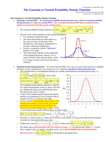
The Gaussian or Normal PDF, Page 4ooIn fact, the words “with 95% confidence” are often not even written explicitly, but are implied. In thisexample, by the way, you can easily calculate the standard deviation. Namely, since 95% confidencelevel is about the same as 2 sigma confidence, 2 9 , or 4.5 .For more stringent standards, the confidence level is sometimes raised to three sigma. For z 3 (three3standard deviations away from the mean), it turns out that A 3 f z dz 0.4987 to four significant0ooo digits. Multiplication by two (because of symmetry) yields the probability that x lies within threestandard deviations from the mean value. Since 2(0.4987) 0.9974, we are 99.74% confident that x lieswithin three standard deviations from the mean.Most engineers and statisticians round down and state simply that there is about a 99.7% confidencelevel that x lies within three standard deviations from the mean. This is in fact a stricter engineeringstandard, called the “three sigma confidence level” or the “99.7% confidence level.”Summary of confidence levels: The empirical rule states that for any normal or Gaussian PDF, Approximately 68% of the values fall within 1 standard deviation from the mean in either direction. Approximately 95% of the values fall within 2 standard deviations from the mean in either direction.[This one is the standard “two sigma” engineering confidence level for most measurements.] Approximately 99.7% of the values fall within 3 standard deviations from the mean in eitherdirection. [This one is the stricter “three sigma” engineering confidence level for more precisemeasurements.]More recently, many manufacturers are striving for “six sigma” confidence levels.Example:Given: The same 1000 temperature measurements used in a previous example for generating a histogram anda PDF. The data are provided in an Excel spreadsheet (Temperature data analysis.xls).To do: (a) Compare the normalized PDF of these data to the normal (Gaussian) PDF. Are the measurementerrors in this sample purely random? (b) Predict howmany of the temperature measurements are greaterthan 33.0oC, and compare with the actual number.Solution:(a) We plot the experimentally generated PDF (bluecircles) and the theoretical normal PDF (red curve) onthe same plot. The agreement is excellent, indicatingthat the errors are very nearly random. Of course,the agreement is not perfect – this is because n isfinite. If n were to increase, we would expect theagreement to get better (less scatter and differencebetween the experimental and theoretical PDFs).(b) For this data set, we had calculated the sample meanto be x 31.009 and sample standard deviation to beS 1.488. Since n 1000, the sample size is largeenough to assume that expected value is nearly equal to x , and standard deviation is nearly equal toS. At the given value of temperature (set x 33.0oC),we normalize to obtain z, namely,A(z) 33.0 31.009 o Cx x xz 1.338o S1.488 C(notice that z is nondimensional). We calculate areaA(z), either by interpolation from the above table or byDesireddirect calculation. The table yields A(z) 0.40955,area1 z and the equation yields A z erf 2 2 1 1.338 erf 0.409552. This means that 40.9552%2 2 of the measurements are predicted to lie between themean (31.009oC) and the given value of 33.0oC (red
oThe Gaussian or Normal PDF, Page 5area on the plot). The percentage of measurements greater than 33.0 C is 50% 40.9552% 9.0448%(blue area on the plot). Since n 1000, we predict that 0.090448 1000 90.448 of the measurementsexceed 33.0oC. Rounding to the nearest integer, we predict that 90 measurements are greater than33.0oC. Looking at the actual data, we count 81 temperature readings greater than 33.0oC.Discussion:o The percentage error between actual and predicted number of measurements is around 10%. This errorwould be expected to decrease if n were larger.o If we had asked for the probability that T lies between the mean value and 33.0oC, the result would havebeen 0.4096 (to four digits), as indicated by the redarea in the above plot. However, we are concernedhere with the probability that T is greater thanNORMSDIST(z)33.0oC, which is represented by the blue area on theplot. This is why we had to subtract from 50% in theabove calculation (50% of the measurements areDesiredgreater than the mean), i.e., the probability that T isareagreater than 33.0oC is 0.5000 – 0.4096 0.0904.o Excel’s built-in NORMSDIST function returns thecumulative area from - to z, the orange-colored areain the plot to the right. Thus, at z 1.338,NORMSDIST(z) 0.909552. This is the entire areaon the left half of the Gaussian PDF (0.5) plus thearea labeled A(z) in the above plot. The desired bluearea is therefore equal to 1 - NORMSDIST(z). Confidence level and level of significanceo Confidence level, c, is defined as the probability thata random variable lies within a specified range ofArea c 1 – values. The range of values itself is called theconfidence interval. For example, as discussed above,we are 95.44% confident that a purely randomArea /2Area /2variable lies within two standard deviations fromthe mean. We state this as a confidence level of c 95.44%, which we usually round off to 95% forpractical engineering statistical analysis.Confidenceo Level of significance, , is defined as the probabilityintervalthat a random variable lies outside of a specifiedrange of values. In the above example, we are 100 –95.44 4.56% confident that a purely randomvariable lies either below or above two standarddeviations from the mean. (We usually round this offto 5% for practical engineering statistical analysis.)o Mathematically, confidence level and level of significance must add to 1 (or in terms of percentage, to100%) since they are complementary, i.e., c 1 or c 1 .o Confidence level is sometimes given the symbol c% when it is expressed as a percentage; e.g., at 95%confidence level, c 0.95, c% 95%, and 1 – c 0.05.o Both and confidence level c represent probabilities, or areas under the PDF, as sketched above for thenormal or Gaussian PDF.o The blue areas in the above plot are called the tails. There are two tails, one on the far left and one on thefar right. The two tails together represent all the data outside of the confidence interval, as sketched.o Caution: The area of one of the tails is only /2, not . This factor of two has led to much grief,so be careful that you do not forget this!
The Gaussian or Normal PDF, Page 3 Linear interpolation: o By now in your academic career, you should be able to linearly interpolate from tables like the above. o As a quick example, let’s estimate A(z) at 2.546. o The simplest way to interpolate, which works for both increasing and decreasing v