WIXLIB

- 5 -is given by p n e z t ( q , j ) . Hence, the algorithm puts j in S , for use when it latercomputes L*,p. More informally, immediately after L,j has been computed it begins“migrating” from one column of A t o another as determined by the values of 7 t e z t ( * , j )(or equivalently the structure of &). The columns visited by L*,j are exactly thosethat must be modified by L*,j. At any point during the factorization, Si n Sj @jfori # j . Consequently, the sets Sj (1 I. j 5 n ) can be stored economically as linked listsusing a single integer array of length n. This is the primary reason for generating thesets Struct(Lj,,) in this manner.2.3. Sources of parallelismAs indicated in [15],there are two sources of potential parallelism in sparse Choleskyfactorization. The first one is in performing cmod operations with the same “updating”column. Suppose Struct(L,,j) {il, i 2 , . .,i,}, with j il i 2 . . . i,. WhenL * j has been computed, columns il, i z , . . ., i, of A have t o be modified by L*,j. Thesecmod’s are independent: they can be performed simultaneously or in any order. Thus,if there are enough processors and if the nonzero entries of L*,j are available t o theseprocessors, the operations crnod(il, j ) , c m o d ( i z , j ) , . . ., cmod(i,, j ) can be performedconcurrently. T h e independence of cmod’s using the same updating column but different target columns has nothing to do with the sparsity of L ; indeed, they are theprimary source of parallelism in a dense column-based factorization.Sparsity in L gives rise t o large-grained parallelism that is not available in a densefactorization. Consider columns L*,k and L * j where j k. We shall say that L,jdepends on L*,k if L,,j cannot be completed until after L*,k has been completed. Whenneither L,,j depends on L l , k nor L * , k depends on L * j , the two columns are said t o beindependent of one another. The column dependencies are very simple when L isdense: since computation of L*,j requires modification of A*,j by a multiple of everycolumn L*,k where IC j , L*,j depends on every such column I,*, To identify columndependencies in the sparse case, we introduce elimination trees.Consider the Cholesky factor L. For each column L*,j having off-diagonal nonzeroelements, we define parent[j] t o be the row index of the first off-diagonal nonzero inthat column; that is, parent[j] n e z t ( j , j ) . For convenience, we define p a r e n t [ j ] tobe j when column L*,j has no off-diagonal nonzeros. The elimination forest of L is agraph 7 with {1,2,. . . , n } as its node set, and an edge connecting i and j if and onlyif j parent[i] and i # j [21,26]. It is also easy to show that 7 is a tree if and onlyif the matrix A is irreducible. Without loss of generality, we will assume from now onthat the given matrix A is irreducible, so that 7 is indeed an elimination tree. Weassume familiarity with the standard terminology associated with rooted trees: e.g.,root, parent, child, ancestor, and descendant. We use the notation 7 [ i ]to denote thesubtree rooted a t node i; that is, I[i]is a tree consisting of i and all of its descendantsin T.

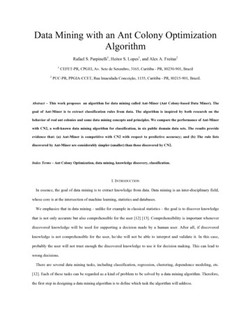
-6-Xxxxx xx xxxxxxxxxxx x XX.XXXXxxxX. .XxxXx xx xxxxxxxxxxx x x X.XXx e e e x xX.OXX.X.X.XX.X0 .XXXXxxxXXxxxx xx xxxxxxxxxxx x XX.XXXXxxx.X.X.xIXxee.xxx.OX0.XXX.OXXX.b.bXeb e0xxeeeea.xxx.OXX.0.Xe.e0 0 .Xxxxx xx xxxxxxxxxxxx XXbXXxX. O Xx e x e x . .XX.XXx .X.xx xxxxxx.0.XXe. e x e e e e x xo x 4 e e e e 6789Figure 2.3: A matrix example defined on a 7 x 7 nine-point grid ordered by nesteddissection. (each x and a refers t o a nonzero in A and a fill entry in I;, respectively.)Consider the cxarnple in Figure 2.3, which contains the matrix and Cholesky factorassociated with a 7 x 7 nine-point grid ordered by the nested dissection algorithm [13].In the figure, each x is a nonzero entry in the matrix A , and each is a fill entry inthe Cholesky factor L. The reader may verify that the tree shown in Figure 2.4 is theelimination tree of the matrix L shown in Figure 2.3.One of the many uses of elimination trees in sparse matrix computation is the analysis of column dependencies in sparse Cholesky factorization. (A survey of eliminationtrees and their applications in sparse matrix computations is contained in [22].) A keyobservation [21,26] is that Strucl(L,,,) C T [ j ] that;is, every k E Struct(L,,*) is adescendant of j in the elirnination tree. Of course, column j of L cannot be completeduntil all columns in Struct( LJ,*) have been completed. Recursive application of this observation t o the descendants of j demonstrates t h a t cnliimn j of L cannot be completediiritjl the columns associated with all descendants of j (i.e., all members of 7 [ j ]- { j } )have been completed. Moreover, L,,J does not depend on any other columns. Hence,columns i and j are independent if and only if 'I [i] and 7 [ j ]are disjoint subtrees. For

- 7-AAFigure 2.4: Elimination tree for the matrix shown in Figure 2.3.

-8example, column 41 in Figure 2.4 depends on columns 22 -- 40, and depends on noother columns of the matrix. Columns 41 and 21 are independent because 7[41] and?-[all are disjoint sirbtrees.2.4. Parallel sparse Cholesky factorizationWe now describe a n algorithm for shared-memory multiprocessor systems that exploitsthese two sources of parallelism. (The algorithm was introduced in [15].) The taskof computing column L,j is referred to as a column task in the computation and isdenoted by T c o l ( j ) . More precisely,TcoE(j): {cmod(j,k) 1 k E S t u t ( L , , jU) }{ c d i u ( j ) } .The parallel algorithm maintains a pool of column tasks, and each processor will beresponsible for performing a subset of these column tasks. The assignment of columntasks t o processors is dynamic. When a, processor is free, it will get a column task fromthe pool, perform the necessary @modoperations, and then carry out the required cdivoperation. When the processor has finished a column task, it will get another columntask from the pool. Efficient implementation of this dynamic scheduling strategy requires that the pool of tasks be made available t o all processors. This is particularlyappropriate for shared-memory multiprocessor systems. This approach usually resiiltsin good load balancing, as might be expected.The parallel algorithm in [15] is presented in Figure 2.5. A few comments on theparallel algorithm are in order. First, note that it is quite similar t o the algorithm inFigure 2.2. Second, we assume that the d a t a reside in a globally-shared memory sothat every processor can access the entire set of data. Third, since every processor willpopping a column task from Q is a critical section and mustaccess the pool of tasksbe performed in a synchronized manner.Fourth, updating an index set S, requires another critical section since S, may besimultaneously updated by more than one processor. In Figure 2.5, we have used twoprimitives, l o c k and unlock, to synchronize this operation. The first primitive, l o c k ,sigiials the beginning of a critical section and allows only one processor t o proceed. Ifthere is already a processor executing the critical section, a second processor attemptingt o enter the same section must wait until the first processor has exited the section.The second primitive, unlock, signals the end of a critical section, and its execution byone processor permits another processor t o enter the critical section. The number ofsynchronization operations required to maintain the pool of tasks is O ( n ) . It is easy t osee that the number of synchronization calls required to update each set "5, is O( lL \).Thus, the total number of synchronization calls required in the parallel algorithm ise,O(lLI).

-9-Global initialization:Q { T c o l ( l ) ,TcoZ(2),.,TcoZ(n)}for j 1 to n dosj -end fore,Work performed by each processor:while Q # 0 dopop T c o l ( j ) from Qwhile column j requires further ernod's doif Sj 0 thenwait until Sj # 0end iflockobtain k from Sjq - n e x t ( j , b )if q 5 n thens, 4" VIend if -unlockcmod(j, Is)end whilecdiw(j)Q ne ,j)if q 5 n then -locks,s, u {jlunlock -end ifend whileFigure 2.5: A parallel sparse Cholesky factorization algorithm for shared-memory multiprocessor machines.

-10 -3. Supernodal Cholesky factorization algorithmsAlthough the results reported in [15] indicated t h a t the parallel algorithm in Figure 2.5achieved good speed-up ratios, the algorithms in Figures 2.2 and 2.5 are far fromoptimal for a t least two important reasons. First, both the sequential and paraUelalgorithms are poor at exploiting some of the hardware features available on advancedcomputer architectures, in particular, the pipelined arithmetic units on current vectorsupercomputers, Second, the number of synchronization operations connected withcritical sections in the parallel algorithm is relatively high.In this section, we discuss the notion of supernodes in the Cholesky factor of asparse symmetric positive definite matrix, and show how these supernodes can be usedt o improve the algorithms in Figures 2.2 and 2.5. In particular, we show how bothdifficulties with the algorithm in [15] can be dealt with by taking advantage of thesupernodal structure.3.1. Notion of supernodesIn the Cholesky factor of a sparse symmetric positive definite matrix, columns with the“same” sparsity structure are often clustered together. Such a grouping of columns isreferred to as a supernode’. We define a supernode of a sparse Cholesky factor L t o bea contiguous block of columns in L , { p , p 1,. . .,p Q - l}, such t h a t Struct( L*,,) Struct(L*,, ,-l) u { p 3- 1,. ., p Q --- 11.* It is quite easy to show that for p 5 i 5 p Q -- 2, Struet(L,,,) S t r c t ( L , , , . - 1U){i 1,. ., p Q - l}. (For details consult [23,24]). Thiis, the columns of the supernode{ p , p -t1, . . .,p 3 q -.-I} have a dense diagonal block and have identical structure belowrow pq - 1. Figure 3.1 shows a set of supernodes for the matrix of Figure 2.3.‘The partition of the columns of E into supernodes is often referred t o as a supernodepart it ion.Apparently, the term “supernode” first appeared in [ 5 ] , although the basic ideabehind the term was used much earlier. For example, the notion of supernodes hasplayed an important role in improving the efficiency of the minimum degree orderingalgorithm [17] and the symbolic factorization process [27]. More recently, supernodeshave been used t o organize sparse numerical factorization algorithms around matrixvector or matrix-matrix operations that reduce memory traffic, thereby making moreeficicnt use of vector registers [3,5] or cache [1,25]. They play such a role in both theserial and the new parallel Cholesky factorization algorithms presented in this section.Note t h a t supernode partitions are not uniquely specified in our definition. Indeed,the choices of a supernode partition depend heavily on the mazimal sets of contigiious ‘It is convenient to denote a column L*,, belonging to a supernode by its column index j . It shouldbe clear by context when 3 i s being used in this manner.

-11 8499x3xx 0e4*e4e e .e** **e* eee.4.*.e4123456789(.exe e x xe e .XX* * e x*.*XX1x e e e x x.ex**e e xxeeXeeeeexxe e e e e e e e .XXeee.eeeee e x x7 8 9 8 1 2 3 4 5 6 7 8 9 3O l 2 3 4 5 6 7 8 940 1 2 3 4 5 6 7 8 9Figure 3.1: Fundamental supernodes in the matrix given in Figure 2.3. (Each x and 0represents a nonzero in A and a fill in L , respectively. Numbers over diagonal entrieslabel supernodes.)

-12 -columns t h a t can be supernodes and from which one or more supernodes can be formed.We have used so-called fundamental supernodes in our algorithms. T h e set K { p , p 1,. . ,p q - l} is a fundamental supernode if K is a maximal subset ofcontiguous columns t h a t forms a supernode for which the following holds: for i I,2,. ., q - 1, the node p 3- i - 1 is the sole child of p -f i in the elimination tree. Thenotion of fundamental supernodes was introduced in [4] and was discussed extensivelyin [23].The fundamental supernodes for our model problem are shown in Figure 3.1.Associated with any supernode partition is a supernodal elimination tree, which isobtained from the elimination tree essentially by collapsing the nodes (colurnns) ineach supernode into a single n d c .The supernodal elimination tree for the partitionin Figure 3.1 is shown in Figure 3.2, superimposed on the underlying elimination tree.The primary reason for using the fundamental supernode partition in this application was pointed out in [23]: it is the coarsest supernode partition for which thesupernode dependencies can be observed in the supernodp elimination tree in a manner strictly analogous t o the way the column dependencies are observed in the nodalelimination tree. Consequently, a fundamental supernode partition can be used morecleanly and naturally in a parallel factorization algorithm, where d a t a dependenciesare of great practical importance. Liu et al. [23] contains a full discussion of this point.Givcn the matrix A , the supernode partition can be obtained by several means.When the ordering of the colurnns and rows of A is a minimum degree or nesteddissection ordering, the partition can be obtained easily as a natural by-product ofthe reordering step. Otherwise, the supernode partition can be obtained directly fromthe structure of L after the symbolic factorization; it can also be obtained before thesymbolic factorization using the algorithm given in [23]. 3.2 Sequential super nodal C holesky factorizationIn this section we describe a left-looking sequential sparse Cholesky factorization algorithm that exploits the supernodal structure in L. T h e algorithm is not new; itsvariants have appeared in 151 and [25]. Let K { p , p I,. . . , p q - 1) be a supernodein L. Consider the computation of L ,3for some j p q .- 1. Suppose column A*,Jhas to be modified by L*,, where i E M . It follows from the definition of supernodest h a t columnwill be modified by aEI columns of pi. In other words, a columnj y q - 1 is either updated by no column of K or every column of K . Thisobservation has some important ramifications for the performance of sparse Choleskyfactorization. Loosely speaking, the columris in a supernode can now be treated asa single unit in the computation. Since the columns in a supernode have the samesparsity structure below the dense diagonal block, modification of a particular columnj p 1- q - I by these columns can be accumulated in a work vector using densevector operations, and then applied t o the target column using a single sparse vectoroperation t h a t employs indirect addressing. Moreover, the use of loop unrolling in the

- 13 -31f44151245891112Figure 3.2: Supernodal elimination tree induced by the fundamental supernodes of thematrix shown in Figure 2.3. Ovals enclose supernodes that contain more than onenode; nodes not enclosed by ovals are singleton supernodes. Bold-face numbers labelsupernodes.

- 14 accumulation, as described in [9], further reduces memory traffic. These issues havebeen addressed in deta.il in [1,3,5,25].In Figure 3.3, we present a siipernodal Cholesky factorization algorithm, whichis quite similar to the orie in Figure 2.2. In Figure 2.2, Si identifies the columns ofL needed t o modify A , j when L * , j is computed. Incorporating supernodes into thealgorithm, we exploit the fact that columns in the same supernode update the sameset of columns outside the supernode. 'Thus, Si will identify the supernodes needed t omodify A , j when L,j is t o be computed. In Figure 3.3, we have adopted the followingnotation. Supernodes are denoted by hold capital letters, and in order t o keep thenotation simple K is t o be interpreted in one of two diflerent senses, depending on thecontext in which it appears. In one context, X is interpreted as the set of columnscomposing the supernode, i.e., K III { p , ; . 1 , . . . , p q - 1). In other lines of thealgorithm, the supernodes are treated as an ordered set of loop indices 1, 2, . . . , K ,. . . , N , where K J if and only if p p', where p and p' are the first columnsof K and J , respectively. This dual-purpose notation is illustrated in Figure 3.1,where the supernode labels are written over the diagonal entries, yet we can still write30 {40,41,42}, for example. We denote both the last supernode and the number ofsupernodes by N .S u p p o s e K { p , p l , .,p q - I } . Wheneverj p q - 1 andZj,p q-l # 0, thetask c m o d ( j , K ) consists of the operations crnod(j,k) where k p , p 1, . . .,p q - 1.If, however, j E K , then c m o d ( j , K ) consists of the operations c m o d ( j , k ) , for k p , p 1,. . . ,j - 1. Suppose L ,e is the last column in a supernode K and let Ij,e # 0.Then n e z t ( j , K ) i s defined t o be n e z t ( j , l ) . Similarly, we define n e z t ( K , K ) t o benext(& e).To reiterate the advantage of exploiting the supernodal structure of L , we note thatM can be accumulated in work storage by a sequencethe operation c m o d ( j , K ) for jof dense vector operations (saxpy using the BLAS terminology [19]), a,fter which theaccumulated column modifications can be applied t o the target column L,,j using asingle column operation that requires indirect addressing. Execution of the operationc m o d ( j , S ) for j E J is even easier, requiring no work storage or indirect addressing. Inboth cases, loop unrolling can be employed to reduce memory traffic, thereby iniproving the utilization of pipelined arithmetic units, especially on vector supercomputers.These capabilities are not available in the "nodal" Cholesky factorization algorithm inFigure 2.2. 3.3. Parallel supernodal C h l e s k yfactorizationAs far as we know, the first attempt t o parallelize a supernodal Cholesky factorizationalgorithm was described in [as]. Using the notation in Figure 3.3, the basic idea in[28] is t o partition the work in c m o d ( j , M )and c m o d ( j , J ) evenly among the availableprocessors. This approach is similar to that employed in the LAPACK project [2],

- 15-for j 1 to N doSj 0end forfor J 1 to N dofor j E J (in order) dofor K E Sj docmod(j, K )q - n e z t ( j , K )if q n thens,end if -s, u W Iend forcmod(j, J )cdiv(j)end forq - n e s t ( J , J )if Q 5 a thens,end if -8, u { J lend forFigure 3.3: A sequential supernodd Cholesky factorization algorithm.

-16 -where, in the interest of software portability and reliability, use of miiltiple processorsoccurs strictly within each call t o some computationally intensive variant of a matrixmatrix multiply (BLAS3) or matrix-vector multiply (BLAS2) kernel subroutine. Henceeach call t o the kernel involves a fork-and-join operation. For large dense m

cmod(j, k) end for Figure 2.1: A sequential sparse Cholesky factorization a.lgorithm. Since the algorithm in Figure 2.1 is column-oriented and the nonzeros of L are stored by columns, its implementation is quite straightforward except for the determination of the structure of row j of L (i.e., Struct(Lj,,)). Instead of computing the structure of