Transcription
6.876 Advanced Topics in Cryptography: LatticesSeptember 16, 2015Lecture 4Lecturer: Vinod VaikuntanathanScribe: Akshay DegwekarIn this class, we will cover The LLL Algorithm. Applications of LLL – Babai’s Algorithm for approximating CVP.2– Exact SVP in 2O(n ) poly(W ) time.– Solving “low density” subset sum problems.1The LLL AlgorithmWe begin describing the algorithm of Lenstra, Lenstra and Lovász for approximating the shortest vector ofa lattice.Theorem 1. Given a basis B Zn n there is a poly(n, WB )-time algorithm for SVP2O(n) , where WBis the length of the bit representation of B; namely, the algorithm returns a vector v L(B) such thatkvk 2O(n) · λ1 (B).The LLL algorithm actually transforms, in polynomial time, the given basis into a “LLL-reduced” basisfor the same lattice. The above theorem holds since a LLL-reduced basis has an important property — itsshortest vector is a 2O(n) -approximation for the shortest vector in entire the lattice. In this lecture we’ll givedefine a LLL-reduced basis and give some intuition for this definition; in the next lecture we’ll describe andanalyze the LLL algorithm itself.1.1LLL-reduced BasisOur goal is to transform the given basis to one with “short” vectors. Consider the case n 2, i.e., B [b1 , b2 ]. Our starting point is the Gram-Schmidt orthogonalization process in which we set b̃1 : b1 andb̃2 : b2 µ21 b̃1 , where µ21 hb2 , b̃1 i/hb̃1 , b̃1 i. Intuitively, b̃2 is the shortest vector we can hope for, sincewe removed all b̃1 ’s components from it (this fact is what make the Gram-Schmidt orthogonal). However,b̃2 / L(B), and thus cannot be in a basis of L(B). To fix this issue, we transform B into the following basis:b01 b and b02 b2 bµ21 e b01 , where b·e means rounding to the closest integer. b02 is the shortest latticevector we can hope for, as we removed all the integer components of b̃1 . Note that when projecting b02 tothe line generated by b01 , then this projection is between b01 /2 to b01 /2. The latter fact also guaranteesthat the resulting basis is “close” to orthogonal — the angle between b01 to b02 is at least 60 degrees. SeeFigure 1 for an example of this transformation.So far we reduced b2 , but left b1 as is. But what if b1 is very long to begin with? there is no guaranteethat the reduced basis is short. At this point we adopt an idea from Euclid’s greatest common divisor (gcd)algorithm: we reduce b2 with respect to b1 as much as we can, then swap the roles of b1 and b2 and repeatthe process. The process will stop when the basis meets the following conditions, which are the definition ofLLL-reduced basis in two dimensions.Definition 2 (LLL-reduced basis in two dimensions). A basis B [b1 , b2 ] is LLL-reduced if1. µ21 1/2.4-1
b02b̃2b2 60 b01 /2b1b01 /2Figure 1: The LLL-reduced basis of [b1 (2, 0), b2 (3, 2)] is [b01 (2, 0), b02 (1, 2)].2. kb2 k kb1 k.2Note that the second condition can be written as b̃2we get the following definition. (1 µ221 ) b̃12. Generalizing for n dimensionsDefinition 3 (LLL-reduced basis). Let δ [1/4, 1]. A basis B [b1 , . . . , bn ] is δ-LLL-reduced if1. µij 1/2 for every 1 i j n.22.b̃i 1 (δ µ2i i,i ) b̃i2for every 1 i n 1.Note that the projection of a (partial) LLL-reduced basis [b1 , . . . , bi 1 , bi , bi 1 ] to Span(b̃i , . . . , b̃n ) is[0, . . . , 0, b̃i , bi 1 µi 1,i b̃i ]. The last two vectors meet the definition of LLL-reduced basis in two dimensions.2The LLL Algorithm2.1LLL-reduced basisTo recap, we defined a δ-LLL reduced basis last classDefinition 4 (δ-LLL-reduced basis). Let δ (1/4, 1). A basis B [b1 , . . . , bn ] is δ-LLL-reduced if1. size-reduced. µi,j 1/2 for every i j.22. Lovász criterion.b̃i 1 (δ µ2i i,i ) b̃i2for every 1 i n 1.To get some intuition for this definition, we look at the 2d variant we saw last class where we said22that kb2 k kb1 k equivalently b̃2 (1 µ22,1 ) b̃1 . We are slightly changing this by adding aδ as a parameter. Geometrically, the criterion looks at the projection of vectors b1 , b2 · · · bn on to theGram-Schmidt vectors. The first few vectors b1 · · · bi 1 project to 0, bi becomes b̃i and bi 1 projects to4-2
b̃i 1 µi 1,i b̃i . So the Lovász criterion compares the norms of these two projected vectors and says thatthe second one is ‘longer’ than the first one, like the 2d case.It is interesting to note that this condition is extremely local and it can be extended to looking at k vectorsat a time to give a 2k time, 2n/k approximation to SVP. We want to argue that finding a LLL-reduced basisis enough to get an approximate shortest vector. n 1 2λ1Lemma 5. If B is a δ-LLL reduced basis, then kb1 k 4δ 1Proof. Since B is δ-LLL reduced, we know that 2b̃i 1 µi 1,i b̃i δ b̃iUsing the fact that the Gram-Schmidt basis is ortogonal, we rearrange the equation to get2b̃i 1Here we substitute the fact that µi 1,i 12 (δ µ2i 1,i ) b̃ito get that2b̃i 12From this we infer that b̃ius the required result.2 (i 1 ( 4δ 1b̃14 )4δ 1) b̃i422. This used in conjunction with λ1 mininb̃iogivesSo, in any LLL-reduced basis, the first vector would be a good approximation to the shortest vector. Itis interestingno to note that this gives us a bit more - we can use the fact that the i-th largest element of theset b̃jgives us a lower bound on λi to get a comparable approximation on λi for all i.j2.2Finding an LLL-reduced basisLemma 5 reduces the problem of getting a 2O(n) approximation to SVP to finding an LLL-reduced basis. Inthis section we describe the LLL algorithm to find a reduced basis and analyze it.123Input Basis b1 , b2 · · · bnwhileCompute b̃1 , b̃2 · · · b̃n afor i 2 to n // Reduction Stepfor j i 1 to 1bi bi ci,j bj qwhere ci,j bµi,j eif i such that b̃i 1 δ µ2i 1,i b̃ib// Swap stepSwap bi and bi 1elseOutput b1 , b2 · · · bna This step does have some issues with runtime - the exact Gram-Schmidt vectors mightkeep getting bigger in terms of bit length. We don’t consider those issues here.b We do not recompute the b̃ ’s again because the Reduction step does not affect b̃ ’s.iiFigure 2: The LLL algorithm4-3
The LLL-algorithm is an iterative algorithm where in each iteration, we first replace the vectors bi ’s by‘approximately’ orthogonal vectors in the lattice obtained from the vectors b̃i ’s. After this, we check if theLovász criterion is violated for any pair of vectors bi , bi 1 . In case of a violation, we swap the two vectorsand continue.Correctness To prove correctness, we need to show that, if the algorithm terminates, then the outputbasis is LLL-reduced.In order to show that µi,j 12 , consider the last iteration. It will not do any swaps and hence thevectors b̃i ’s will remain unchanged in the iteration.On the other hand, because we subtract ci,j ’s, the values old old 1/2. Note that this relies on the factof µi,j ’s changes. Namely µnewand hence µnewi,j µi,j µi,ji,jthat we are decrementing j in step 2 of the algorithm. The Lovász criterion is satisfied by termination – ifit was not satisfied for some i, then we would swap bi and bi 1 and iterate again.Termination The termination is a potential argument. We define a non-negative potential function φ(B)for any basis and then show that it was not too large to begin with and that each iteration reduces thisfunction by a constant.QLet φ(B) i φi (B) whereφi (B) det(L(b1 , b2 · · · bi )) Where the determinant for non full rank matrices is defined as det(B) det( B B). Another way towrite it would beφi (B) b̃1 · b̃2 · · · b̃iObservation 6. φ(B) is not too large to begin withφ(Binit ) nYkb1 k · kb2 k · · · kbi k max(kbi k)O(n2)ii 1So, log(φ(Binit )) poly(n, W ) where W is the bit length of the vectors. We also know that φ(B) 1because of the fact that we are dealing with integer lattices and each potential φi can be interpreted as thei-dimensional volume enclosed by the vectors b1 , b2 · · · bi .Observation 7. The reduction step does not change the potential functionThis is evident by looking at φi (B) b̃1b̃2 · · · b̃i and observing that the reduction step leavesb̃i ’s invariant.Observation 8. The swap step reduces φ by a constant factor.Proof. Let us say that bi and bi 1 were swapped. This only affects the value of φi (B) because changingorder of vectors does not affect the determinant.The old value of φi is, φold b̃1 · b̃2 · · · b̃i while the new value is φnew b̃1 · b̃2 · · · b̃i 1 ·iib̃i 1 . We see that the component of b̃i 1 orthogonal to the span of b1 , b2 · · · bi 1 is b̃i 1 µi 1,i b̃i . So,b̃i 1 µi 1,i b̃iφnewφnew iold oldφφib̃i δSo as long as δ 1 is a fixed constant, we know that the potential function decreases by a constantfactor.Combining the observations we see that the algorithm has to terminate in time poly(n, W ).4-4
3ApplicationsThe LLL algorithm has many applications - the most famous one being factoring polynomials over rationals.It also gives us an algorithm for finding the exact shortest vector - while the algorithm takes exponentialtime, it was the first algorithm to solve exact SVP for a fixed dimension.3.12)Computing Shortest Vectors in 2O(nTimeCorollary 9 (Exact SVP). There is an exact SVP algorithm running in time 2O(n2)PProof. To show this we consider an LLL-reduced basis B. Consider a shortest vector v i ci bi . We wantto say that ci 2O(n) and hence by iterating over ci ’s and returning the smallest vector would give us a22O(n ) algorithm. PPConsider v i ci bi v i c̃i b̃i . We look at the last i such that ci is non-zero. Then ci c̃ibecause it is the only coefficient contributing in the b̃i direction. Since kb1 k kvk ci b̃i , we get that4)(i 1)/2 because b̃ici ( 4δ 13.22i 1 ( 4δ 1b̃14 )2.Babai’s Algorithms for Approximate CVPCorollary 10 (Babai’s Algorithm for Approximate CVP). Let B be a reduced LLL-basis and y be the inputvector. There are two variants of the algorithm 1. Babai’s rounding algorithm - We find the representationof y in the real span of B and output the rounded coefficients. Succinctly, output B B 1 y2. Babai’s nearest plane algorithm - The algorithm works iteratively. We consider the hyperplane H Span(b1 · · · bn 1 ) and its translations - bn H, 2bn H and so on and find the one closest to y, thenproject y on H and recurse.References[1] Divesh Aggarwal and Daniel Dadush and Oded Regev and Noah Stephens-Davidowitz. Solving the Shortest Vector Problem in 2n Time Using Discrete Gaussian Sampling: Extended Abstract. STOC 2015.[2] Lenstra, A.K. and Lenstra, H.W.jun. and Lászlo Lovász. Factoring polynomials with rational coefficients.Math. Ann. 19824-5
The LLL algorithm has many applications - the most famous one being factoring polynomials over rationals. It also gives us an algorithm for nding the exact shortest vector - while the algorithm takes exponential time, it was the rst algorithm to solve exact SVP for a xed dimension. 3.1 Computing Shortest Vectors in 2))) (4) (4) 1 1 2. 1