Transcription
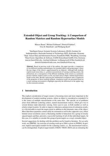
Extended Object and Group Tracking: A Comparison ofRandom Matrices and Random Hypersurface ModelsMarcus Baum , Michael Feldmann†, Dietrich Fränken‡,Uwe D. Hanebeck , and Wolfgang Koch† Intelligent Sensor-Actuator-Systems Laboratory (ISAS), Institute forAnthropomatics, Karlsruhe Institute of Technology (KIT), Karlsruhe, Germany†Dept. Sensor Data and Information Fusion, Fraunhofer FKIE, Wachtberg, Germany‡Data Fusion Algorithms & Software, EADS Deutschland GmbH, Ulm, Germanymarcus.baum@kit.edu, {michael.feldmann @eads.com, uwe.hanebeck@ieee.orgAbstract: Based on previous work of the authors, this paper provides a comparisonof two different tracking methodologies for extended objects and group targets, wherethe true shape of the extent is approximated by an ellipsoid. Although both methodsexploit usual sensor data, i.e., position measurements of varying scattering centers, thedistinctions are a consequence of the different modeling of the extent as a symmetricpositive definite random matrix on the one hand and an elliptic random hypersurfacemodel on the other. Besides analyzing the fundamental assumptions and a comparisonof the properties of these tracking methods, simulation results are presented based ona static tracking environment to highlight especially the differences in the update stepfor the extension estimate.1IntroductionThe explicit consideration of target extents is becoming more and more important in thedevelopment of modern tracking systems, where an object is considered as extended if itis the source of multiple measurements at the same time. The specific set of problemsarises from different scattering centers, named measurement sources, which give rise toseveral distinct radar detections varying, from scan to scan, in both number as well asrelative origin location. In order to improve robustness and precision of estimation results,it is felt desirable to track the target extent in addition to the kinematic state of the object.More than these quantities cannot safely be estimated as well in the (opposite) case, wherelimited sensor resolution causes a fluctuating number of detections for a group of closelyspaced targets and thus, prevents a successful tracking of (all of) the individual targets. Inthis case, it is suitable to consider this group of point targets as a single extended object.Several suggestions for dealing with this problem can be found in literature. For an earlywork, see [DBP90]. An overview of existing work up to 2004 is given in [WD04]. In general, implicit and explicit models for the scattering centers, i.e., the measurement sources,can be distinguished. Explicit target models [VIG04, VIG05, IG03] aim at estimating the
location of the measurement sources in addition to kinematics of the object. These approaches require data association and are not treated in this paper. An implicit model forthe target extent assumes that the measurement sources are generated independently according to an internal state of the object that reflects the extent. An example for an implicitmodel is a so-called spatial distribution model, where each measurement source is assumedto be an independent random draw from a probability distribution [GGMS05, GS05].In this paper, we discuss two different tracking methods for extended object tracking,where the measurement sources are modeled implicitly and the true physical extensionis approximated by an ellipsoid. Ellipsoidal shapes are highly relevant for real worldapplications, as an ellipsoid provides useful information about the target orientation andspatial extent. Here, the focus is on track maintenance, while estimation under uncertainobservation-to-track association in the possible presence of missed detections and falsealarms is considered out of scope.The first tracking method considered in this paper is based on the use of symmetric positive definite (SPD) random matrices and has been introduced in [Koc08]. Therein, an SPDrandom matrix to describe the ellipsoid is the counterpart of a random vector representingthe centroid. The decisive point for tracking of extended objects in [Koc08] is the special interpretation of usual sensor data, whereupon each measurement is considered as ameasurement of the centroid scattered over object extension. This implicit neglect of anystatistical sensor error has caused some further investigations and developments to honorthe fact that both sensor error and extension contribute to the measurement spread [FF09].Hence, we employ two approaches: the original one of [Koc08] as well as the advancedone of [FF09]. The second tracking method is based on a random hypersurface model(RHM), which has been introduced in [BNH10]. An Elliptic RHM specifies the relativeMahalanobis distance of a measurement source to the center of the target object by meansof a one-dimensional random scaling factor. In order to avoid the treatment of an SPD matrix for the ellipsoid, the kinematic state of the extended object is supplemented with thenon-zero entries of the Cholesky factorization of the inverse SPD matrix. By this means,all parameters describing the corresponding ellipsoid are contained in one random vector.This paper analyzes the fundamental assumptions of these three tracking approaches andprovides a comparison of the properties of the two different methods. It is completedby simulation results based on a static tracking environment to highlight especially thedifferences in the update step for the extension estimate.2General Problem DescriptionThe considered problem is to track the kinematics and the extent of an unknown extendedobject in the (x, y)-plane based on Cartesian position measurements corrupted by additivestochastic noise. It is assumed that there is a random number of nk noisy position measurements arising from nk unknown measurement sources in each scan k, i.e., the objectextension is not directly observable. More formally, the unknown measurement source attime step tk is denoted with zjk . In this paper, the measurement ykj is the observation of zjk
Measurementsource modelMeasurementmodelStochastic noise v k Measurement source MeasurementFigure 1: Model of the generation process for one measurement.according to a specific measurement model (see Figure 1) given byykj zjk wkj ,(1)where wkj denotes additive white Gaussian noise. The goal is now to estimate and tracka summarizing shape, e.g., an ellipsoid, which reflects the extent and shape of the measurement sources. In doing so, the major challenge is that the measurement sources aregenerated according to an unknown model. For instance, a group of point targets may generate at each time step only a discrete set of measurement sources. A spatially extendedobject, however, may generate measurement sources that stem from a continuous domain,i.e., the target surface. For ellipsoidal shapes, two different methods have been recentlyproposed: SPD random matrices (see Section 3) and Elliptic RHMs (see Section 4).3Method I: Random MatricesIn order to achieve robust tracking of extended objects and group targets, the two approaches in [Koc08, FF09] supplement the corresponding conventional (kinematic) trackfile with a random variable representing the physical extent, which is approximated by anellipsoid with the result that the target extent can be described by a symmetric positivedefinite (SPD) matrix. Such a matrix-valued random variable is named a random matrixand invokes matrix-variate distributions [GN99].3.1Measurement Likelihood FunctionAccording to the proposal in [Koc08, FF09], the physical extent represented by an SPDrandom matrix Xk is considered besides the kinematic state of the centroid described bythe random vector xTk [rTk , ṙTk ] with the spatial state component rk , where d dim(rk )is also the dimension of Xk . Now, it is assumed that in each scan k there is a randomnumber of nk independent position measurementsykj Hxk wkj(2)with the measurement source zjk b Hxk and the measurement matrix H [Id , 0d ]. Furthermore, expected sensor reports are considered as measurements of the centroid scatteredover the extent so that, having regard to the measurement noise variance R, the noise wkj
is assumed to be a zero-mean normally distributed random vector with variance zXk R.The scaling factor z enables us to account for a difference between an assumed normalspread contribution of the extent and a possibly more realistic assumption such as, e.g.,a uniform distribution of varying scattering centers over an object of finite extent. Withk(denoting the set of the nk meathis, the likelihood to measure the set Yk : {ykj }nj 1surements in a particular scan k) given both kinematic stateobject extent as well asQnandkthe number of measurements reads p(Yk nk , xk , Xk ) j 1N (ykj ; Hxk , zXk R).Thereupon, the computation of the mean measurement and the measurement spreadyk nk1 Xyj ,nk j 1 kYk nkXj 1(ykj yk )(ykj yk )T(3)is considered as a preprocessing step to rewrite the likelihood function according top(Yk nk , xk , Xk ) N (yk ; Hxk , (zXk R)/nk ) W(Yk ; nk 1, zXk R) ,(4)where W(X; m, C) denotes the Wishart density [GN99] of an SPD random matrix X withexpected SPD matrix mC.3.2Bayesian InferenceIn this context, a tracking algorithm is an iterative updating scheme for conditional probability densities p(xk , Xk Y k ) of the joint object state (xk , Xk ) at each time tk given theaccumulated sensor data Y k : {Yκ , nκ }kκ 0 . For this reason, the derivation of explicitfilter equations is based on the application of the concept of conjugate priors—the verysame concept that constitutes one possible way of deriving the well-known Kalman filterequations for point source tracking—to the measurement likelihood function for receivingupdate equations and then complemented with an evaluation of the Chapman-Kolmogorovtheorem for obtaining a recursive Bayesian estimation cycle.It appears that for the likelihood p(Yk nk , xk , Xk ), no conjugate prior can be found thatis both independent of R and analytically traceable. For this reason, any statistical sensorerror is ignored in [Koc08], i.e., setting R 0, to derive a closed-form solution within aBayesian framework on the supposition that the spread of the measurements is dominatedby the extent. This means, by implication, that the estimator of [Koc08] effectively estimates extent plus sensor error, while an equal Kalman gain (for the kinematics estimate)is effective in each spatial dimension because the filter cannot judge the quality of themeasurements.In view of these observations, the alternative approach in [FF09] adapts the original approach in [Koc08] using some careful approximations to honor the fact that both sensorerror and extent contribute to the measurement spread. In detail, the updated estimate ofthe centroid kinematics is determined by using standard Kalman filter equations with themean measurement yk and an approximation of the true innovation covariance. However,this way of proceeding requires knowledge of the true extent Xk so that it is assumed that
SelectionMeasurementmodelSamplingp(sk)01Scaling factorStochastic noise wkskFigure 2: Random Hypersurface Models.the predicted extent is not too far away from the truth and can be used as a replacement forXk where needed.In both approaches, the update of the extent estimate is carried out by a weighted sum ofthe predicted extent, the measurement spread, and a dyadic product, which evaluates thedifference between the expected and the measured centroid position. The latter enables anupdate of the extent estimate even in the case of a single measurement. The differencesbetween both approaches are due to the particular weighting of the individual quantities,where [FF09] uses matrix-valued scaling to compensate the effects of the statistical sensorerror on the measurements.4Method II: Elliptic Random Hypersurface Models (RHMs)The development of Elliptic RHMs for extended object tracking [BNH10] has been drivenby the idea to estimate the smallest enclosing ellipse of the extended target.An Elliptic RHM [BH09] is a specific measurement source model (see Figure 1) that assumes each measurement source to lie on a scaled version of the true ellipse describingthe target (see Figure 2). The scaling factor is specified by an independent random drawfrom a one-dimensional probability density function. It can be interpreted as the (relative)distance of the measurement source from the target center with respect to the Mahalanobisdistance induced by the true ellipse. It is important to note that all five ellipse parameterscan be estimated based on measurements generated from an Elliptic RHM.The probability density of the scaling factor has to be specified in advance. It was proven in[BNH10] that, if the measurement sources are drawn from a uniform spatial distributionon the entire ellipse surface, the squared scaling factor is uniformly distributed on theinterval [0, 1]. Hence, a uniformly distributed squared scaling factor is a rational choice.Note that the converse is not true, i.e., a uniformly distributed squared scaling factor doesnot necessarily lead to a uniform distribution on the entire ellipse. There are many spatialdistributions, which yield a uniformly distributed squared scaling factor.Another natural choice is to assume the random scaling factor to be Gaussian distributed[BH09]. A Gaussian distributed scaling factor is for instance useful when measurementsources at the border of the ellipse are more probable than measurement sources in thecenter of the ellipse.
In order employ an Elliptic RHM, a suitable parametric representation of an ellipse has tobe selected. The center of the ellipse is modeled with the random vector rk . In order toavoid the treatment of positive semi-definite random matrices, the shape of the ellipse, i.e.,the physical extension of the extended object, is represented with the Cholesky decomposition of the SPD matrix (Xk ) 1 Lk · LTk , where a0Lk : k(5)ck bkis a lower triangular matrix with positive diagonal entries.The state vector turns out to be of the form xk [rTk , lTk , . . .]T with lk [ak , bk , ck ]T .Note that xk may also contain further state variables, e.g., for the kinematics of the target.The ellipse specified by xTk is given by the setEk {z z R2 and g(z, xk ) 1}with shape function g(z, xk ) : (z rk )T · (Lk · LTk ) · (z rk ). The scaled version ofEk with scaling factor sk is given byEks {z z R2 and g(z, xk ) s2k } .4.1Measurement Likelihood FunctionThe measurement likelihood function can be constructed by formulating a measurementequation, which relates the unknown state xk to the measurement ykj . If there would beno measurement noise, i.e., ykj zjk , the measurement equation would beg(zjk , xk ) s2k 0 ,(6)which maps the unknown parameters xk to the pseudo-measurement 0 with additive noiseterm s2k . Unfortunately, the measurement source is not known, only its noisy measurementykj zjk wkj is given. If the measurement ykj is inserted in (6), a deviation w̄kj on theright hand side may be obtained, i.e., we obtain the measurement equationg(ykj , xk ) s2k w̄kj .(7)Actually, w̄kj is a random variable, because ykj depends on the measurement noise. Theprobability distribution of w̄kj can be approximated with a Gaussian distribution by meansof moment matching. For this approximation, the true parameters of the ellipse must beknown. Hence, similar to the alternative random matrix approach [FF09], the true parameters are substituted with its current estimate. For the detailed formulas see [BNH10].4.2Bayesian InferenceA measurement update with the measurement equation (7) can in general be performedwith a nonlinear state estimator. For both uniformly und Gaussian distributed scaling
factors s2k , closed-form expressions for the first two moments of the updated estimate canbe derived (see [BNH10]). For this purpose, the probability distribution of the randomvector [xTk , g(ykj , xk ) w̄kj ]T is approximated with a Gaussian distribution by analyticmoment matching. In case of a Gaussian distributed squared scaling factor s2k , the updatedestimate then results from the Kalman filter equation. For a uniformly distributed squaredscaling factor s2k , the updated estimate results from calculating the first two moment of atruncated Gaussian distribution.Again, the measurement update step is complemented with an evaluation of the ChapmanKolmogorov theorem for obtaining a recursive Bayesian estimation cycle.5ComparisonThis section highlights the differences of both tracking methods for tracking extendedobjects. For this purpose, we directly compare several properties that characterize bothmethods. Subsequently, the main differences of both methods are discussed.5.1Method I: Random MatricesRepresentation of an ellipse. The basic assumption to model the extent by an ellipsoidcorresponds with earlier work (see, e.g., [Bla86, DBP90]), but the novelty of [Koc08,FF09] is that it relies on the joint estimation of centroid kinematics and physical extent.For that purpose, an SPD random matrix to describe this ellipsoid is the counterpart of arandom vector representing the centroid and enables us to derive closed-form expressionsfor the Bayesian inference mechanism.Interpretation of an elliptic extent. For a group of closely spaced targets, the obtainedtracking results are comparable to the sample mean and the (scaled) sample covariance ofthe group members.Modeled measurement source distributions. By means of the scaling factor z, it ispossible to account for a difference between an assumed normal spread contribution of theextent and a possibly more realistic assumption like, e.g., a uniform distribution of varyingscattering centers over an object of finite extent X. In this instance, recalling the idea ofsecond order moment matching leads to z 1/4 as an appropriate choice for the scalingfactor because the variance of the varying measurement sources is equal to X/4.Processing of measurements. Both random matrix approaches update the state estimatesby exploiting indirect measurement parameters: the mean measurement yk and the measurement spread Yk . This means that all nk measurements are processed in one updatestep, where the computation of yk and Yk can be considered as a preprocessing step.Other target shapes. The use of SPD random matrices confines the target shape modelingto ellipsoids, where an eigenvalue corresponds to the squared semi-axis length.
Estimation of measurement noise. In the case of point source targets, it is possible forboth approaches to estimate an unknown measurement error covariance (i.e., setting R 0 in the alternative approach [FF09]) by means of the dyadic product, which evaluates thedifference between the expected and the measured centroid position.5.2Method II: Elliptic RHMRepresentation of an ellipse. An Elliptic RHM represents an ellipse by means of a parameter vector consisting of the center and the vectorized Cholesky decomposition of the SPDshape matrix. The uncertainty about the parameter vector of the ellipse is modeled with aGaussian distribution. However, RHMs are not restricted to this particular representationof the parameters.Interpretation of an elliptic extent. An Elliptic RHM aims at estimating the smallestenclosing ellipse of the extended target. One can say that the parameters of the ellipseare estimated such that the squared relative Mahalanobis distance from the center to themeasurement sources is uniformly distributed. For a group of closely spaced targets, thecenter of this ellipse does not have to be the sample mean and the shape matrix does nothave to coincide with the (scaled) sample covariance of the group members.Modeled measurement source distributions. An Elliptic RHM with uniformly distributed squared scaling factor is able to estimate the correct parameters of an ellipse on whichthe measurement sources are drawn from a uniform distribution. However, an EllipticRHM with uniformly distributed squared scaling factor models in fact many spatial distributions on the ellipse.Processing of measurements. The measurement update step for Elliptic RHM does notmake use of a preprocessing step. Independent measurements can be processed sequentially. Moreover, the computational complexity is linear in the number of received measurements.Other target shapes. RHMs are modular. The parametric representation of the shapeand the inference mechanism can be exchanged. RHMs can even be generalized to othershapes by means of employing a proper implicit shape function.Estimation of measurement noise. In general, an Elliptic RHM could also be used forestimating the measurement noise of a point target. An Elliptic RHM can also be seen asa special type of noise, which specifies the random distance of a disturbance. In order toestimate Gaussian noise, the corresponding probability distribution of the scaling factorwould have to be employed. However, this has not been investigated so far.5.3DiscussionThe first main difference between the two methods is the interpretation of the ellipsoidalextent. While for a group of point source targets, the tracking results of the random matrix
approaches are comparable to the sample mean vector and the (scaled) sample covariancematrix of the group members, Elliptic RHMs aim at estimating the smallest enclosingellipse of the target group. However, if the measurement sources are drawn uniformlyover an ellipse, both tracking methods estimate the same ellipse. The random matrixapproaches are also capable of estimating Gaussian distributed measurement sources. Onthe other hand, Elliptic RHMs are able to employ Gaussian distributed scaling factors. Thesecond main difference is the representation of an ellipse. The random matrix methodemploys an SPD random matrix for the elliptic shape and a random vector for the center.Elliptic RHMs, as presented in this paper, make use of a Gaussian distributed randomvector that consists of the center and the shape.All together, it highly depends on the particular application and requirements, whichmethod for extended object tracking should be used.6Simulation ResultsThis section presents simulations results, which validate the insights about the two trackingmethods worked out in the previous sections.The presented simulations treat only non-moving targets because the main difference (ofall discussed approaches) is the way the target extent is modeled. For concrete trackingexamples, we refer the reader to [Koc08, FF09] and [BNH10].6.1Static Extended ObjectThe first example is a static extended object, where the extended object in fact has anelliptic shape. Moreover, the measurement sources are uniformly distributed on the ellipsesurface, which is a natural assumption if there is no information about the target available.According to Section 5, both methods are capable of estimating the correct parameters ofthe ellipse in this case. In order to validate these results, we have performed three differentsimulations, where the measurement sources are sampled uniformly from the true ellipse.The number of measurements nk in each scan k was Poisson-distributed with mean 5. Themeasurement noise is set to low (σ 20 m), medium (σ 50 m), and high (σ 75 m)compared to the size of the ellipse (with diameters 300 m and 200 m). The estimationresults are shown Figure 3. There, it can be seen that both methods, i.e., SPD randommatrices and Elliptic RHMs, provide accurate estimation results for all noise levels. Theoriginal random matrix approach [Koc08], which does not incorporate the measurementnoise, overestimates the true ellipse.
[Koc08]0.20.1y / km 000 0.1 0.1 0.1 0.2 0.2 0.2 0.2 0.100.1 0.2 0.10.2x / km 0.1 0.2 0.10.2y / km y / km 00 0.1 0.1 0.2 0.2 0.200.1 0.2 0.10.2x / km 0.1 0.2 0.10.2y / km y / km 00 0.1 0.1 0.2 0.2 0.200.1x / km 0.20.20.1 0.1 0.2 0.10.1[BNH10]0.20.100x / km [FF09]0.20.1y / km 0x / km [Koc08]0.20.20.1 0.1 0.2 0.10.1[BNH10]0.20.100x / km [FF09]0.20.1y / km 0x / km [Koc08]0.2[BNH10]0.20.1y / km 0.1y / km [FF09]0.2 0.2 0.100.1x / km 0.2 0.2 0.100.10.2x / km Figure 3: Simulation results for a static extended object, where the left column of figures summarizesthe estimation results (black) of the original random matrix approach [Koc08] after 100 scans, themiddle column the results of the alternative approach [FF09], and the right column the results of theElliptic RHM approach [BNH10]. Shown are also the track initialization (green), the true ellipse(blue) and the accumulated measurements (red) of 100 scans with σ 20 m (top row), σ 50 m(middle row), and σ 75 m (bottom row).6.2Static Group of Point TargetsIn the second example, the extent of a static group of 16 point targets is to be estimated.Each group member produces exactly one noisy measurement (σ 15 m) at each timestep. This example emphasizes that both tracking methods have a different interpretationof an ellipse. In fact, they estimate a different summarizing shape. While the trackingmethod using random matrices precisely estimates the sample mean and the scaled samplecovariance matrix, the Elliptic RHMs aim at estimating the smallest enclosing ellipse ofthe target group. The methods estimate different quantities because the underlying modelof the extended target is different. The estimation results are depicted in Figure 4. Note
[Koc08]0.20 0.1 0.100.1x / km 0.20.10 0.1 0.1[BNH10]0.2y / km 0.1y / km y / km 0.1[FF09]0.200.1x / km 0.20 0.1 0.100.10.2x / km Figure 4: Simulation results for a static group of point targets, where the left part summarizes theestimation results (black) of the original random matrix approach [Koc08] after 50 scans, the middlepart the results of the alternative approach [FF09], and the right part the results of the Elliptic RHMapproach [BNH10]. Shown are also the scaled ellipse (light blue) of the sample covariance for therandom matrix approaches, the true point target positions (blue), the accumulated measurements(red) of 50 scans, and the track initialization (green).that the estimated ellipse of the advanced random matrix approach [FF09] (that accountsfor measurement noise) as well as Elliptic RHMs do not depend on the measurement noise,as it is filtered out. However, the size of the estimated ellipse of the original random matrixapproach [Koc08] (that neglects measurement errors) would increase with an increasingmeasurement error.7Conclusion and Future WorkIn this work, a comparison of two tracking methods for extended targets has been given.The first method models the target extent with an SPD random matrix and the second oneemploys a so-called random hypersurface model. After a unified description of the twomethods, we have given a detailed comparison of the different assumptions and properties of the methods. We have shown that the main difference lies in the interpretation ofan elliptic extent. Both methods estimate an ellipse that summarizes the shape of the extended target. However, the quantity the estimated ellipse summarizes is different for bothmethods. Actually, the desired interpretation remains the user’s choice because it highlydepends on the particular application.As already mentioned in the introduction, the explicit consideration of target extents is becoming more and more important in the development of modern tracking systems. However, extended object tracking is still a relatively new research area with a variety of openproblems and challenges. In order to embed extended object tracking methods into a realworld tracking system, the proposed methods have to be extended to deal with clutter andmulti-extended objects. In this context, it is also necessary to develop methods for splittingand merging tracks consisting of extended objects or groups of point targets.In real-world scenarios, one typically has to deal with nonlinear measurement models for
which both methods would have to be adapted. Finally, it would be interesting to developmethods that are able to estimate more complex shapes than ellipses.References[BH09]M. Baum and U. D. Hanebeck. Random Hypersurface Models for Extended ObjectTracking. In Proc. 9th IEEE International Symposium on Signal Processing and Information Technology (ISSPIT 2009), Ajman, United Arab Emirates, 2009.[Bla86]S. Blackman. Multiple-Target Tracking with Radar Applications. Artech House, 1986.[BNH10]M. Baum, B. Noack, and U. D. Hanebeck. Extended Object and Group Tracking withElliptic Random Hypersurface Models. In Proc. 13th Int. Conf. on Information Fusion(Fusion 2010), Edinburgh, United Kingdom, 2010.[DBP90]O. Drummond, S. Blackman, and G. Petrisor. Tracking clusters and extended objectswith multiple sensors. In Proc. SPIE Conf. Signal & Data Processing of Small Targets,Orlando, Florida, 1990.[FF09]M. Feldmann and D. Fränken. Advances on Tracking of Extended Objects and GroupTargets using Random Matrices. In Proc. 12th Int. Conf. on Information Fusion (Fusion2009), Seattle, Washington, 2009.[GGMS05] K. Gilholm, S. J. Godsill, S. Maskell, and D. Salmond. Poisson Models for ExtendedTarget and Group Tracking. In Proc. SPIE Conf. Signal & Data Processing of SmallTargets, San Diego, California, 2005.[GN99]A. K. Gupta and D. K. Nagar. Matrix Variate Distributions. Chapman & Hall/CRC,1999.[GS05]K. Gilholm and D. Salmond. Spatial Distribution Model for Tracking Extended Objects.IEE Radar Sonar Navig., 152(5):364–371, 2005.[IG03]N. Ikoma and S. J. Godsill. Extended Object Tracking with Unknown Association,Missing Observations, and Clutter using Particle Filters. In IEEE Workshop on Statistical Signal Processing, St. Louis, Missouri, 2003.[Koc08]W. Koch. Bayesian Approach to Extended Object and Cluster Tracking using RandomMatrices. IEEE Trans. Aerosp. Electron. Syst., 44(3):1042–1059, 2008.[VIG04]J. Vermaak, N. Ikoma, a
Mahalanobis distance of a measurement source to the center of the target object by means of a one-dimensional random scaling factor. In order to avoid the treatment of an SPD ma-trix for the ellipsoid, the kinematic state of the extended object is supplemented with the non-zero entries of the Cholesky factorization of the inverse SPD matrix.