WIXLIB

Bahig Journal of the Egyptian Mathematical Society(2019) 27:3Page 4 of 122. Worst case: this case occurs if the value of n is large and m is small. Therefore, thenumber of elements that belong to the array GrAr is large. So, the running time ofDHS algorithm is O(n x log m), where x n.3. Average case: the authors in [19] do not specify the value of n and m in this case.The running time of the DHS algorithm is O(n x log m), where x n.Comments on DHS algorithmIn this part, we provide two main comments about the DHS algorithm. The first category of comments is related to the theoretical analysis of the DHS algorithm; the second category of comments is related to the data generated in the practical study.For the first category, we found that the running times for the DHS algorithm havethe following three notes.The first note is that the running time calculated for the best case is correct when mis small; the running time calculation is not correct when n is small. When n is smalland m is large, the number of repetitions in the input array is very small in general.Therefore, most of the elements belong to the GrAr array. This situation implies thatthe DHS algorithm uses the quick sort algorithm on the GrAr array. Therefore, therunning time of the third phase is O(n log n), not O(n).Example 1 Let n 10, m n2 100, and the elements of A is well distributed as follows:127718343563456721298989104635It is clear that the value of n is small compared with m. Therefore, in general, thenumber of elements that belong to the EqAr array is very small compared with theGrAr array that contains most of the input elements.The second note is that the calculated running time for the worst case is not correct ifthe value of n is large and m is small. This situation implies that the number of repetitionsin the input array is large because the n elements of the input array belong to a smallrange. Therefore, the maximum number of elements belonging to the GrAr array is lessthan m, say α. On the other hand, the array EqAr contains n α elements. Therefore, thestatement “the number of elements belong to the GrAr array is large” [19] is not accurate.It should be small since m is small. Therefore, the calculated running time for the worstcase of the DHS algorithm, O(n x log m), is not accurate in the general case.Example 2 Let m 4, n m2 16 and A is given as follows11213143546171819110 11 12 13 14 15 161111211It is clear that the number of non-repeated elements is 3 and the GrAr array containsonly 3 different elements, 2, 3, and 4; the EqAr array contains 13 elements from 16.The third note is that no determination when the average case occurs, which is whythe running time is O(n x log m).

Bahig Journal of the Egyptian Mathematical Society(2019) 27:3For the second category, the data results in [19] for the three cases reveal how thatthe percentages of elements in the EqAr array, repeated elements, is at least 65%, whichis too much and do not represents the general or average cases. This situation meansthat the input data used to measure the performance of DHS algorithm do not represent various types of input. For example, in the average case, n 100,000 and the rangeof elements equals 100,000, the number of elements in the EqAr array is 70,030 [19].Complexity analysis of DHS algorithmIn this section, we study the complexity of the DHS algorithm using another method ofanalysis. The DHS algorithm is based on dividing the elements of an input array intomany slots; each slot contains elements in a specific range. Therefore, we mainlyanalyze the DHS algorithm based on the relation between the size of the array, n, andthe domain of the elements in the array, m. There are three cases for the relation between n and m.Case 1: O(m) O(n). In this case, the range of values for the elements of the inputarray is small compared with the number of elements in A. This case can be formed asA (a1, a2, , an), where ai m and m n. We use big Oh notation to illustrate thatpffiffiffithe difference between n and m is significant. For example, let m ¼ n and m log nand if n 10,000, then m 100 and 4, respectively.Case 2: O(m) O(n). In this case, the range of the values for the elements of the inputarray is equal to the number of elements. This case can be formed as A (a1, a2, ,an), where ai m, n m, and m α n β such that α and β are constant. For example,let m 2n and m n 25; if n 1000, then m 2000 and 1025, respectively.Case 3: O(n) O(m). In this case, the range of the values for the elements of the inputarray is greater than the number of elements. This case can be formed as A (a1, a2, , an), where ai m, m n. For example, let m nk , where k 1. If n 100 and k 3,then m 1,000,000.Now, we study the complexity of the DHS algorithm in terms of three cases.Case 1: O(m) O(n). The value of m is small compared with the input size n; thearray contains many repeated elements. In this case, the maximum number of slots ism, and there is no need to map the elements of the input array to n slots such as mapping sort algorithm [20], where the index of the element ai is calculated using the equation: ⌊((ai Min(A)) n)/(Max(A) Min(A))⌋.The solution to this case can be found using an efficient previous sorting algorithmcalled counting sort (CS) algorithm [6]. Therefore, there is no need to use the insertionsort, quick sort, and merge sort algorithms as in [19, 20] to sort un-repeated elements.The main idea of the CS algorithm is to calculate the number of elements less than theinteger i [1, m]. Then, we use this value to allocate the element aj in a correct locationin the array A, 1 j n. The CS algorithm consists of three steps. The first step of theCS algorithm starts with scanning the input array A and computing the number of repetitions each element occurs within the input array A. The second step of the CS algorithm is to calculate, for each i [1, m], the starting location in the output array byupdating the array C using the prefix-sum algorithm. The prefix-sum of the array C isPto compute C½i ¼ ij¼1 C½ j . The final step of the CS algorithm allocates each i [1, m]and its repetition in the output array using the array C.Page 5 of 12

Bahig Journal of the Egyptian Mathematical Society(2019) 27:3Page 6 of 12Additionally, the running time of the CS algorithm is O(n m) O(n), because O(m) O(n). The running time of the CS algorithm does not depend on the distribution ofthe elements, uniform and non-uniform, over the range m. Also, the CS algorithm isindependent of how many repeated and unrepeated elements are found in the inputarray.The following example illustrates how to use the CS algorithm in this case; there isno need to distribute the input into two arrays, EqAr and GrAr, as in the DHSAlgorithm.Example 3 Let m 5, n m2 25, and the elements of the input array A as in Fig. 1a.As a first step, we calculate the repetition array C, where C[i] represents the number ofrepetitions of the integer i [1, m] in the input array A as in Fig. 1b. It is clear that thenumber of repetition for the integer “1” is 6; the integer “4” has zero repetition. In thesecond step, we calculate the prefix-sum of C as in Fig. 1c, where the prefix-sum forPC[i] is equal to ij¼1 C½ j . In the last step, the integer 1 is located from positions 1–6;the integer 2 is located from positions 7–14 and so on. Therefore, the output array isshown as in Fig. 1d.Remark Sometimes the value of m cannot fit in memory because the storage of themachine is limited. Then, we can divide the input array into k ( m) buckets, where thebucket number i contains the elements in the range [(i 1)m/k 1, i m/k], 1 i k. Fora uniform distribution, each bucket contains n/k elements approximately. Therefore,the running time to sort each bucket is O(n/k k). Hence, the overall running time isO(k(n/k k)) O(n k2) O(n). For non-uniform distributions, the number of elementsPin each bucket i is ni such that ki¼1 ni ¼ n. Therefore, the overall running time is O(n k) O(n).Case 2: O(m) O(n). The value of m is approximately equal to the input size n. If theelements of the array are distributed uniformly, then the number of repetitions for theelements of the array is constant. In this case, we have two comments about the DHSalgorithm. The first comment is that there is no need to construct two different arrays,GrAr and EqAr. The second comment is that there is no need to use the quick sort algorithm in the sorting because we can sort the array using the CS algorithm.If the distribution of the elements for the input array is non-uniform, then the number of repetitions for the elements of the array is varied. Let the total number 192021222324255 2 2 5Input array A.123252321161718192021222324252 2 3 3Sorted array A.33335555531441556 0 5Count array C.34514 20 20 25(c) Prefix-sum for C.123456789101112111111222222(d)131415Fig. 1 Tracing of the CS algorithm in case of O(m) O(n). a Input array A. b Count array C. c Prefix-sum forC. d Sorted array A

Bahig Journal of the Egyptian Mathematical Society(2019) 27:3Page 7 of 12repetitions for all the elements of the input array be φ(n). Therefore, the array EqArcontains φ(n) elements; the array GrAr contains n φ(n) elements. The running timefor executing the DHS algorithm is O(n (n φ(n)) log (n φ(n)) ), where the first termrepresents the running time for the first two stages and the second term represents applying the quick sort algorithm on the GrAr array. In the average case, we have n/2 repeated elements, so the running time of the DHS algorithm is O((n/2) log (n/2) ) O(nlog n). In this case, the CS algorithm is better than the DHS algorithm. On the otherside, if φ(n) n, then the running time of the DHS algorithm is O(n).Example 4 Let m 30, n 25. Fig. 2 shows how the CS algorithm can be used insteadof the DHS algorithm in the case of a uniform distribution.Case 3: O(n) O(m). The value of m is large compared with the input size n, so theelements of the input array are distinct or the number of repetitions in the input arrayis constant in general. The DHS and CS algorithms are not suitable for this case. Reasons for not considering these strategies include the following:1. All of these algorithms require a large amount of storage to map the elementsaccording to the number of slots. For example, if m n2 and n 106 (this value issmall for many applications), then m 1012 which is large.2. If the machine being used contains a large amount of memory, then the runningtimes of the DHS algorithm are O(n log n). But the main drawbacks of the DHSalgorithm are (1) the output of the second hashing function is not unique; (2) theequations used to differentiate between repeated elements and non-repeated elements are not accurate which means that there is an element with certain repetitions and another element without repetition have the same visual indicesgenerated by the suggested equations. Therefore, merge sort and quick sort are better than the DHS algorithm.3. In the case of CS, the algorithm will scan an auxiliary array of size m to allocatethe elements at the correct position in the output. Therefore, the running time isO(m), where O(m) O(n). If m n2, then the running time is O(n2) which isgreater than merge sort algorithm, O(n log n).1234567891011121314151617 181920212223242526 4 6 18 1 8 13 20 11 12 26 4 30 21 25 23 7 5 29 19 15 2 11 17 4(a) Input array A.12345678910 11 12 13 14 15 16 17 18 19 20 21 22 23 24 25 26 27 28 29 3011031111002110(b)10 1 1 1Count array C.1101012001112345678910 11 12 13 14 15 16 17 18 19 20 21 22 23 24 25 26 27 28 29 301225678999 11 12 13 13 14 14 15 16 17 18 19 19 20 20 21 23 23 23 24 25(c) Prefix-sum for 11121315 17 18 19Sorted array A.2021232526262930(d)1516Fig. 2 Tracing of the CS algorithm in case of O(m) O(n). a Input array A. b Count array C. c Prefix-sum forC. d Sorted array A

Bahig Journal of the Egyptian Mathematical Society(2019) 27:3From the analysis of the DHS algorithm for the three cases based on the relation between m and n, there is a previous sorting algorithm that is associated with less timecomplexity than the DHS algorithm.Performance evaluationIn this section, we studied the performance of the DHS and CS algorithms from a practical point of view based on the relation between m and n for the two cases, O(m) O(n) and O(m) O(n). Note that both algorithms are not suitable in the case of O(n) O(m).Platforms and benchmarks settingThe algorithms were implemented using C language and executed on a computer consisting of a processor with a speed of 2.4 GHz and a memory of 16 GB. The computerran the Windows operating system.The comparison between the algorithms is based on a set of varied benchmarks toassess the behavior of the algorithms for different cases. We build six functions asfollows.1. Uniform distribution [U]: the elements of the input are generated as a uniformrandom distribution. The elements were generated by calling the subroutinerandom() in the C library to generate a random number.2. Duplicates [D]: the elements in the input are generated as a uniform randomdistribution. The method then selects log n elements from the beginning of thearray and assigns them to the last log n elements of the array.3. Sorted [S]: similar to method [U] such that the elements are sorted in increasingorder.4. Reverse sorted [RS]: similar to method [U] such that the elements are sorted indecreasing order.5. Nearly sorted [NS]: similar to [S]; we then select 5% random pairs of elementswaps.6. Gaussian [G]: the elements of the input are generated by taking the integer valuefor the average of four calling for the subroutine random().In the experiment, we have three parameters affecting the running time for both algorithms. The first two parameters are the size of the array n and the domain of the input m; the third parameter is the data distribution (six benchmarks). Based on therelation between n and m, say O(m) O(n), we fixed the size of the array n and adopteddifferent values of m, mi, such that mi O(m) O(n). For example, let n 108, and thevalues of m are m1 106, m2 105, m3 104, m4 103, and m5 102. For each fixedvalue of n and mi, we generated six different input data values based on the six benchmarks (U, D, S, RS, NS, G). For each benchmark, the running time for an algorithmwas the average time of 50 instances, and the time was measured in milliseconds.Therefore, the running time for the algorithm, Alg, using the parameters n, m and acertain type of data distribution, is given by the following equation.Page 8 of 12

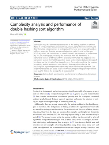
Bahig Journal of the Egyptian Mathematical Society(2019) 27:3nm501 X1 Xt i ðn; mi ; dd; Alg Þnm i¼1 50 j¼1Page 9 of 12!where mi is one of the values for m such that mi satisfies either O(m) O(n) or O(m) O(n). In the experiment, if n 10x, then 102 mi 10x-2.nm is the number of different values for mi. In the experiment, if n 10x, then nm x-3, because 102 mi 10x-2.dd is the type of data distribution used in the experiment, and the value of dd isone of six benchmarks (U, D, S, RS, NS, G).Alg is either the CS or DHS algorithm.ti is the running time for the Alg algorithm using the parameters n, mi, and the datadistribution dd.In our experiments for both cases, we choose the value of n equal to 108, 107, 106,and 105, because the running times for both algorithms are very small when n is lessthan 105.Experimental resultsThe results of implementing the methodology to measure the running time of the CSand DHS algorithms considering all parameters that affect the execution times areshown in Figs. 3 and 4. Each figure consists of four subfigures (a), (b), (c), and (d) for n 105, 106, 107, and 108, respectively. Also, each subfigure consists of six pairs of bars.Each pair of bar represents the running times for the CS and DHS algorithms using a416CSDHS3Time (milliseconds)Time (milliseconds)CS210[U][D][S][RS][NS]Distribution of Data(a) n 10584[U][D][S][RS][NS]Distribution of Data(b) n 101500DHSTime (milliseconds)Time [G]6120090060030000[U][D][S][RS][NS]Distribution of Data(c) n 107[G][S][RS] [NS]Distribution of Data(d) n 108[G]Fig. 3 Running time for the CS and DHS algorithms in case of O(m) O(n). a n 105. b n 106. c n 107.d n 108

Bahig Journal of the Egyptian Mathematical SocietyCSPage 10 of 1260DHSTime (miliseconds)Time (miliseconds)40(2019) ]Distribution of Data(a) n 105[G]4000Time (milliseconds)Time ution of Data(b) n 106[G][S][RS][NS]Distribution of Data(d) n n of Data(c) n 107[G][U][D]Fig. 4 Running time for the CS and DHS algorithms in case of O(m) O(n). a n 105. b n 106. c n 107.d n 108certain type of data distribution. Fig. 3 illustrates the running times for the CS andDHS algorithm in the case of O(m) O(n) and shows that the running time for the CSalgorithm is faster than for the DHS algorithm for all values of n and benchmarks. Thedifference in running time between the algorithms varies from one type of data distribution to another. For example, the running time for the CS algorithm using the sixbenchmarks are 7.7, 9.7, 8.2, 9.8, 8.2, and 6.1 milliseconds; while the running times forthe DHS algorithm using the same benchmarks are 11.2, 12.4, 10.6, 15, 13.9, and 14.1milliseconds in the case of n 106. In general, the maximum difference between thetwo algorithms occurs in the case of a Gaussian distributionSimilarly, Fig. 4 illustrates the running times for the CS and DHS algorithm in thecase of O(m) O(n) and shows that the running time for the CS algorithm is fasterthan for the DHS algorithm for all values of n and benchmarks.Table 1 lists data pertaining to the performance improvements of the CS algorithm intwo points of view (i) range of improvements, and (ii) mean of improvements. In the caseof a range of improvements, we fix the size of the array n and calculate the percentage ofimprovement for each benchmark. Then, we record the range of improvements from theminimum to maximum values as in the second and fourth columns in Table 1 forTable 1 Range of improvements for the CS and DHS algorithmsnO(m) O(n)O(m) O(n)Range of improvementsAverage improvementsRange of improvementsAverage –53.8%35.4%821–47%28.1%24.8–43.5%33.6%10

Bahig Journal of the Egyptian Mathematical Society(2019) 27:3O(m) O(n) and O(m) O(n), respectively. In the case of the mean of improvements, wetake the mean value for the percentage of improvements for all data distributions, as inthe third and fifth columns. The results of applying these measurements are as follows.1. In the case of O(m) O(n), the CS algorithm performed 45–80%, 21.5–56.5%, 20–57%, and 21–47% faster than the DHS algorithm for n 105, 106, 107, and 108,respectively. For example n 108, the percentage of improvements for CSalgorithm for data distribution: [U], [D], [S],

(DHS) algorithm, has been shown to exceed the quick sort algorithm in performance by 10-25%. In this paper, we study this technique from the standpoints of complexity analysis and the algorithm's practical performance. We propose a new complexity analysis for the DHS algorithm based on the relation between the size of