Transcription
Exercise 4. Watershed and Stream Network DelineationGIS in Water Resources, Fall 2012Prepared by David Tarboton, Utah State UniversityPurposeThe purpose of this exercise is to illustrate watershed and stream network delineation based on digitalelevation models using the Hydrology tools in the ArcGIS Geoprocessing toolbox. In this exercise, youwill perform drainage analysis on a terrain model for the San Marcos Basin. The Hydrology tools areused to derive several data sets that collectively describe the drainage patterns of the basin.Geoprocessing analysis is performed to recondition the digital elevation model and generate data onflow direction, flow accumulation, streams, stream segments, and watersheds. These data are then beused to develop a vector representation of catchments and drainage lines from selected points that canthen be used in network analysis. This exercise shows how detailed information on the connectivity ofthe landscape and watersheds can be developed starting from raw digital elevation data, and that thisenriched information can be used to compute watershed attributes commonly used in hydrologic andwater resources analyses.Learning objectives Identify and properly execute the geoprocessing tools involved in DEM reconditioning.Describe and quantitatively interpret the results from DEM reconditioning as a special case ofquantitative raster analysis.Construct profiles using 3D Analyst.Create and edit feature classes.Identify and properly execute the sequence of Hydrology tools required to delineate streams,catchments and watersheds from a DEM.Evaluate and interpret drainage area, stream length and stream order properties from TerrainAnalysis results.Develop a Geometric Network representation of the stream network from the products ofterrain analysis.Use Network Analysis to select connected catchments and determine their propertiesDo an online watershed delineationComputer and Data RequirementsTo carry out this exercise, you need to have a computer which runs ArcGIS 10.1 and includes the SpatialAnalyst and 3D Analyst extensions. The data are provided in the accompanying zip file, Ex4Data.zipavailable at ip. The data files used in theexercise consist of a DEM grid for the San Marcos Basin in Texas from the National Elevation Dataset andstream and watershed data from the National Hydrography Dataset NHDPlus. If you want to do similar1
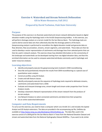
work in a different location you will need to download this data from these data sources. URL's forthese and other data sources were provided in Lecture 4.Data description:Ex4Data.zip should be unzipped and saved in a folder where you will do your work. In this exercise thefolder C:\Users\dtarb\Scratch\Ex4 has been used. The unzipped contents of Ex4Data.zip are illustratedbelow:The geodatabase SanMarcos.gdb contains the following data:Raster analyses such as watershed and stream network delineation are best performed in a consistentprojected spatial reference system (or projection). This is because calculation of slope, length and areaare involved and these are best done in linear (not geographic) units consistent with the elevation units.In this exercise to expedite matters for you the data has all been projected into the NAD 1983 TexasCentric Mapping System Albers.prj spatial reference.In the SanMarcos geodatabase the BasemapAlbers feature dataset contains the four necessary featureclasses. Watershed is the set of HUC 12 watersheds within the San Marcos 8 digit HUC 12100203extracted from the watershed boundary dataset in Exercise 2. Basin is the San Marcos 8 digit HUC12100203 boundary obtained by dissolving the HUC 12 watersheds. Flowline is a subset of NHDPlusflowlines that cover the San Marcos Basin and surrounding area. USGSGage is a set of USGS streamgages within the San Marcos Basin, similar to what was developed in exercise 2.2
There is also a raster smdem that contains the digital elevation model for this region obtained from theNational Elevation dataset. This DEM is equivalent to the DEM you worked with in Exercise 3, exceptthat it has a smaller cell size (30 m) appropriate for this analysis and has been projected to the NAD1983 Texas Centric Mapping System Albers spatial reference being used in this exercise.The exercise is divided in to the following activities that each comprise a sequence of steps1. DEM Reconditioning2. Hydrologic Terrain Analysis3. Network analysisBefore we startSelect Customize ExtensionsSelect the Spatial Analyst and 3D analyst extensions. We will be using both of these during the exercise.3
DEM ReconditioningDEM reconditioning is a process of adjusting the DEM so that elevations direct drainage towards thevector information on stream position, which in this case are the blue line stream features obtainedfrom NHDPlus. DEM reconditioning is only suggested when the vector stream information is morereliable than the raster DEM information. This may not be the case here, but reconditioning is donenevertheless to illustrate the process. DEM reconditioning as done here involves a sequence of ArcGISgeoprocessing functions. The strategy is to first convert vector stream features to a raster dataset ofgrid cells on the streams that has exactly the same dimensions (rows, columns, cell size) as the DEMraster. This exposes you to a number of new geoprocessing tools (Feature to Raster, Greater Than,Reclassify) as well as Environment Settings to control raster cell size, extent and snapping. Then theEuclidean distance from each grid cell to the nearest stream is calculated and a Map Algebra expressionused to perform the reconditioning which involved lowering the elevation of all grid cells along thestreams by 20 units and grid cells near the streams by a value that tapers from 10 to 0 units based onthe distance from 0 out to 500 units. The results are then visualized using 3D Analyst. By doing this youget some experience using the ArcGIS geoprocessing tools to derive new spatial data from the originalDEM and vector streams and a small glimpse into the powerful geospatial analytical capability that thesefunctions enable.1. Feature to Raster.Open ArcMap. Click on theicon to add data. In the dialog box, navigate to the location of thedata; select both the BasemapAlbers feature dataset and smdem raster containing the DEM for the SanMarcos and click on the “Add” button. The data provided will be added to the map display.Click on thesearch icon on the standard toolbar to open the ArcGIS search window. Enter featureto raster and click on the search magnifying glass. This is a way to find tools if you do not know whichtoolbox they are in. You have to however know something about their name or a word used indescribing their functionality.Click on the Feature to Raster tool. Select Flowline as the Input features. Use Field COMID (all we needhere is some unique number). For output raster designate the name FlowlineRaster in the4
SanMarcos.gdb. Note that you can save Rasters in a Geodatabase, which is sometimes a convenientway to keep them organized. Click on the Environments button.In Environment Settings expand Output Coordinates and select Same as Layer "smdem". ExpandProcessing Extent and select Extent same as "smdem" and Snap Raster as "smdem". Click OKClick OK on Environment Settings. Notice that back on the Feature to Raster tool the output cell sizenow inherits the value 30 from the snap raster. Click OK on the Feature to Raster tool.5
The result is a FlowlineRaster that represents the flowlines as a raster with value corresponding to theirCOMID. The particular field used was somewhat arbitrary as we really just need a value by which toidentify stream grid cells. If you zoom in and adjust the layers displayed you can see that the result is aset of grid cells that have been created from the flow lines. The grid values on these lines are all largeinteger numbers because that is what the COMID is.Save your ArcMap document as Ex4.mxd2. Threshold using Greater Than to obtain stream raster.To identify whether a grid cell is part of a stream or not, we use the greater than function to obtain abinary (0, 1) raster of stream cells. Locate the Greater Than tool (using the search window) and enterthe following input, click OK. This picks out all the cells with COMID’s in them.6
The result is a raster with value 1 for stream cells and no data elsewhere.To use in calculations below, we need 0's not NoData off the streams, so let's reclassify this. Locate theReclassify tool (using the search window) and enter the following input, click OK. (It does not matterwhich of Reclassify (3D Analyst) or Reclassify (Spatial Analyst) tools you select. They are functionally thesame, just associated with different extension licenses)7
The result is a raster where NoData values have been replaced by 0's. If you have trouble getting thisfunction to operate correctly, hit the Classify button and open and close this window. This seems toenter a new set of Old Values 0-1 in the Old Values column, first row, and then the function works ok.3. Distance to streamsSearch on distance and open the Euclidean Distance tool. Set Flowline as the input feature anddesignate distance as the output raster in the SanMarcos.gdb.Click on Environments and as before set Output Coordinates same as smdem and Processing Extentsame as smdem and Snap Raster to smdem.8
The result is a grid giving distances to the streams that looks a bit like the inside of an intestine (sorry!).9
4. AGREE Reconditioning with Map Algebra.The distance and FlowlineReclas grids contain the information required to do an AGREE like (see Lecture9 slide 33 and rdi/research/agree/agree.html)reconditioning of the DEM to burn in the streams. Save your Map document in case of an error,because it is easy to get an error in the next step which requires that the expression below beconstructed precisely. Open the Raster Calculator on Map Algebra and construct the followingexpression (use the keys in the visual keypad to construct this expression and don’t attempt to type ityourself because the spacing between the characters in the expression is important to getting this towork properly).The output is saved in a raster named smrecon (San Marcos reconditioned) in the SanMarcos.gdb. TheMap algebra expression is interpreted as follows10
Note that the units involved are elevation units which in this case are m. Distance was constructedusing map units, which are also m here.If you have trouble with this step, pick up the required grid from the backup 2012/Ex4/smrecon.zip5. 3D AnalystLet's use Raster calculator and 3D Analyst to see what this has produced.Use raster Calculator to evaluate the following expressionThe worm like result shows how the DEM has been altered to reduce values along the streams.11
Select Customize Toolbars 3D Analyst to display the 3D Analyst toolbarSet the target layer in the toolbar to smrecon and click on the interpolate line buttonon the map across a stream. Then click on the Create Profile Graph buttonbutton) to obtain a profile graph.12. Draw a line(under the Point Profile
Repeat the procedure with target layers "smdem" and "diff". It seems that you have to redraw the lineeach time, but with a bit of fiddling you can illustrate the effect of reconditioning on the DEM.To turn in:1. Screen captures that illustrate the effect of DEM Reconditioning. Show the location where youmade a cross section as well as the DEM cross sections with and without reconditioning.Open the attribute table of FlowlineReclas and find the number of grid cells that were mapped asstream cells. Given that the size of each grid cell is 30 m estimate the length of channels in the area13
defined by the smdem grid as this number of cells times 30 m. Actually this is an over estimate becauseFlowlineReclas approximates the Flowline feature class using a stair step approach. Nevertheless theresult is a rough estimate useful for cross checking. Use the total number of grid cells in theFlowlineReclas raster dataset, and grid cell area to estimate the total area and take the ratio to estimatethe drainage density (Length of Channels/Total Area).To turn in:2. Number of stream grid cells in FlowlineReclas and estimates of channel length and drainagedensity.Open the Layer Properties of the diff raster and find the average amount of "earth" removed by thereconditioning process. Multiply this by the total area to get the total volume of "earth" removed. Thecross section of "earth" removed was a swath 1000 m wide along the streams with triangular crosssection (illustrated in a profile graph) going down to 10 m and a spike 30 m wide going down to 20 m.Calculate the area of this cross section and multiply it by the length of channels to get another estimateof the volume of "earth" removed by this reconditioning.To turn in:3. Volumes of earth removed estimated from (a) layer properties of diff and (b) from estimates ofchannel length and cross section area. Comment on the differences.Hydrologic Terrain AnalysisThis activity will guide you through the initial hydrologic terrain analysis steps of Fill Pits, calculate FlowDirection, and calculate Flow Accumulation (steps 1 to 3). The resulting flow accumulation raster thenallows you to identify the contributing area at each grid cell in the domain, a very useful quantityfundamental to much hydrologic analysis. Next an outlet point will be used to define a watershed as allpoints upstream of the outlet (step 4). Focusing on this watershed streams will be defined using a flowaccumulation threshold within this watershed (step 5). Hydrology functions will be used to defineseparate links (stream segments) and the catchments that drain to them (steps 6 and 7). Next the14
streams will be converted into a vector representation (step 8) and more Hydrology toolboxfunctionality used to evaluate stream order (step 9) and the subwatersheds draining directly to each ofthe eight stream gauges in the example dataset (step 10). The result is quite a comprehensive set ofinformation about the hydrology of this watershed, all derived from the DEM.1. FillThis function fills the sinks in a grid. If cells with higher elevation surround a cell, the water is trapped inthat cell and cannot flow. The Fill function modifies the elevation value to eliminate these problems.Select Spatial Analyst Tools Hydrology Fill. Set the input surface raster as smrecon and outputsurface raster as fel in SanMarcos.gdb.Press OK. Upon successful completion of the process, the “fil” layer is added to the map. This processtakes a few minutes.2. Flow DirectionThis function computes the flow direction for a given grid. The values in the cells of the flow directiongrid indicate the direction of the steepest descent from that cell.Select Spatial Analyst Tools Hydrology Flow Direction.Set the inputs as follows, with output "fdr".Press OK. Upon successful completion of the process, the flow direction grid “fdr” is added to the map.15
To turn in:4. Make a screen capture of the attribute table of fdr and give an interpretation for the values inthe Value field using a sketch.3. Flow AccumulationThis function computes the flow accumulation grid that contains the accumulated number of cellsupstream of a cell, for each cell in the input grid.Select Spatial Analyst Tools Hydrology Flow Accumulation.Set the inputs as followsPress OK. Upon successful completion of the process, the flow accumulation grid “fac” is added to themap. This process may take several minutes for a large grid, so take a break while it runs! Adjust thesymbology of the Flow Accumulation layer "fac" to a classified scale with multiplicatively increasingbreaks that you type in, to illustrate the increase of flow accumulation as one descends into the gridflow network. Use 8 classes and hit the “Classify” Button to enable you to select “Manual” method andto type in your class breaks into the window in the lower right hand corner.16
17
After applying this layer symbology you may right click on the "fac" layer and Save As Layer FileThe saved Layer File may be imported to retrieve the symbology definition and apply it to other data.Add the SanMarcos Basin feature class. This shows the outline of the San Marcos basin. Change thesymbology so that this is displayed as hollow and zoom in on the outlet in the South East corner. Turn18
off unnecessary layers so that you can see the basin feature class on top of the fac layer. Use theidentify tool to determine the value of "fac" at the point where the main stream exits the area definedby the San Marcos Basin polygon. This location is indicated in the following figure.The value obtained represents the drainage area in number of 30 x 30 m grid cells. Calculate thedrainage area in km2.Also examine the edges of the San Marcos Basin as represented by the Basin feature class. Note theconsistency between this basin boundary and streams as represented by flow accumulation. Notice alsohow, apart from cutting off a number of meanders, there is generally good agreement between theFlowline feature class and flow accumulation grid. This is a result of the DEM reconditioning that wasperformed.To turn in:5. Report the drainage area of the San Marcos basin in both number of 30 m grid cells and km2 asestimated by flow accumulation.Add the SanMarcos Watershed feature class. This shows the outline of the HUC 12 subwatersheds inthe San Marcos basin. Change the symbology so that this is displayed as hollow and zoom in on theoutlet in the South East corner. Use the identify tool to find the HU 12 NAME of the subwatershedright at the outlet of the San Marcos Basin.19
Use the identify tool to determine the value of "fac" at the point where the main stream enters andexits the area defined by this most downstream subwatershed. Subtract the entering fac value from theexiting fac value to determine the area of this subwatershed. Compare your result to the area reportedin the ACRES and Shape Area attributes of this feature. The Shape Area attribute was calculatedautomatically by ArcGIS when this feature class was created and is in the units consistent with the LinearUnit of this feature class, meters in this case, so area is m2.To turn in:6. Report the name of the most downstream HUC 12 subwatershed in the San Marcos Basin.Report the area of the most downstream HUC 12 subwatershed determined from flowaccumulation, from the ACRES attribute and from Shape Area. Convert these area values toconsistent units. Comment on any differences.4. Isolating our WatershedRather than working with the whole grid, we now want to focus only on the area of the San MarcosWatershed upstream of where flow leaves the Basin feature class. Lets define an outlet point there tohelp us.Open Catalog and right click on SanMarcos\BaseMapAlbers New Feature Class20
Set the Name as Outlet and Type as Point Features. Click Next.Leave the coordinate system as default (inheriting from the Feature Dataset it is going in to) and clickNext. Click Finish at the last screen without changing any of the fields.Now let's use the Editor to create an outlet point in this feature class. Click on the Editor Toolbar buttonon the standard toolbar to activate the Editor toolbar21
Click on Editor Start Editing. Zoom right in on the outlet at the bottom right where flowaccumulation exits the area. Make sure that the Outlet layer is turned on so that it appears in theCreate Features list. Using the Create Features button on the Editor Toolbar with Outlet clickedcarefully place a point at the desired outlet locationClick Editor Stop Editing. Respond Yes to the Save Edits prompt.You should now have a new outlet point feature at your designated outlet.Select Spatial Analyst Tools Hydrology Watershed. Set the inputs as follows and click OK.22
The result should be a Watershed grid that has the value 1 over the area upstream from the outlet pointas evaluated from the flow direction field. Be careful to call this result Wshed not Watershed because itwill get mixed up with the Watershed feature class that you already have in the Geodatabase5. Stream DefinitionLet's define streams based on a flow accumulation threshold within this watershed.Select Spatial Analyst Tools Map Algebra Raster Calculator and enter the following expression,using the name Str for the output raster.The result is a raster representing the streams delineated over our watershed.6. Stream LinksThis function creates a grid of stream links (or segments) that have a unique identification. Either a linkmay be a head link, or it may be defined as a link between two junctions. All the cells in a particular linkhave the same grid code that is specific to that link.23
Select Spatial Analyst Tools Hydrology Stream Link. Set the inputs as follows and click OK.The result is a grid with unique values for each stream segment or link. Symbolize StrLnk with uniquevalues so you can see how each link has a separate value.7. CatchmentsThe Watershed function also provides the capability to delineate catchments upstream of discrete linksin the stream network.Select Spatial Analyst Tools Hydrology Watershed. Set the inputs as follows. Notice that theInput raster pour point data is in this case the StrLnk grid. Click OK.24
The result is a Catchments grid where the subcatchment area draining directly to each link is assigned aunique value the same as the link it drains to. This allows a relational association between lines in theStrLnk grid and Area's in the Catchments grid. Symbolize the Catchments grid with unique values so youcan see how each catchment has a separate value.8. Conversion to VectorLet's convert the raster representation of streams derived from the DEM to a vector representation.Select Spatial Analyst Tools Hydrology Stream to Feature. Set the inputs as follows. Note that Iput the output in the BaseMapAlbers feature dataset.25
Note here that we uncheck the Simplify polylines option. The simplification can cause streams to "cutcorners" that will result in errors when they are later on matched up with values on an underlyingstream order grid during the process of determining stream order.The result is a linear feature class "DrainageLine" that has a unique identifier associated with each link.Select Conversion Tools From Raster Raster to Polygon. Set the inputs as followsThe result is a Polygon Feature Class of the catchments draining to each link. The feature classesDrainageLine and CatchPoly represent the connectivity of flow in this watershed in vector form and willbe used later for some Network Analysis, that is enabled by having this data in vector form.26
To turn in:7. Describe (with simple illustrations) the relationship between StrLnk, DrainageLine, Catchmentsand CatchPoly attribute and grid values. What is the unique identifier in each that allows themto be relationally associated?9. Strahler Stream OrderRun Spatial Analyst Tools Hydrology Stream Order with inputs as follows.The result is a Raster StrahlerOrder that holds Strahler Order values for each grid cell. Let's nowassociate these with the streams represented by DrainageLine.Locate the Zonal Statistics as Table (Spatial Analyst) tool and run it with inputs as followsThe result is a Table "OrderTable" that has zonal statistics from the StrahlerOrder grid corresponding toeach link in the StrLnk grid. Open the DrainageLine attribute table. Select Table Options Add Field.Specify the name StrahlerOrder and leave other properties at their default. (Strahler Orders are smallinteger numbers that should fit in a Short Integer data type)27
Select Table Options Joins and Relates Join, then specify the Join data as followsRespond No to the prompt about indexing.28
The DrainageLine table now displays many more columns because it has included all the columns fromOrderTable. Since the Strahler Order is the same for each link, the fields MIN, MAX, MEAN, MAJORITY,MINORITY, MEDIAN all hold the same value, the stream order and any one of these can be copied intothe StrahlerOrder field we just created.Right Click on the StrahlerOrder field header and select Field Calculator. Click Yes to the warning aboutworking outside an edit session, then double click on the OrderTable.MIN field so that the FieldCalculator displays as follows and click OK.Notice that the StrahlerOrder field is now populated with the minimum OrderTable.MIN values.Remove all Joins from the DrainageLine table.Symbolize the DrainageLine feature class using Strahler Stream Order for color and line width.29
To turn in:8. A layout showing the stream network and catchments attractively symbolized with scale, title andlegend. The symbology should depict the stream order for each stream.10. Stream Gauge SubwatershedsIt is often necessary to delineate watersheds draining to specific monitoring points on the streamnetwork, such as stream gages. Let's do this. If necessary add the USGSGage feature class. This is astream gauge feature class similar to that used in previous exercises. Zoom in close to one of the gages.You will see that although close, the gages do not lie exactly on the streams.Use Spatial Analyst Tools Hydrology Snap Pour Point with the following input30
This results in a raster of pour points close to each gage but on the stream as defined by flowaccumulation.Use Spatial Analyst Tools Hydrology Watershed with the following inputThis results in subwatersheds delineated to each stream gage. These may be used with zonal functionsto evaluate properties of the subwatersheds draining to these gauges.To turn in:31
1. Indicate the field in the gages table that is associated with values in the wshedG. Give the areain number of grid cells and km2 of each gauge subwatershed. Add these as appropriate to givethe total area draining to each gauge and compare to the DA SQ MILE values from the USGS forthese gauges.Network AnalysisSome of the real power of GIS comes through its use for Network Analysis. A Geometric Network is anArcGIS data structure that facilitates the identification of upstream and downstream connectivity. Herewe step through the process of creating a geometric network from the vector stream networkrepresentation obtained above, and then use it to determine some simple aggregate information.Zoom in to near the Outlet and select Start Editing on the Editor Tool. Sometimes you encounter awarning that certain layers are not editable. If this happens close and re-open ArcMap. Click on the EditTool (red circle below) then click on the outlet point and drag it until it lines up with the DrainageLineEndpoint as shown below. It should snap right on.Select Stop Editing and Save on the Editor.Now open the Catalog window and right click on BaseMapAlbers New Geometric Network32
Click Next on the New Geometric Network screen. Enter the name SanMarcosNet, then click Next.Select the features DrainageLine and Outlet. These will be used to create a Geometric Network. ClickNext.33
At the prompt to Select roles for the network feature class switch the role under Sources and Sinks forOutlet to Yes. This will be used as a Sink for the network. This is a location that receives flow. ClickNext.Do not add any weights at the prompt about weights, just click Next. Click Finish at the summaryprompt. The result is a Geometric Network SanMarcosNet that can be used to perform networkoperations34
Select Customize Toolbars Utility Network Analyst from the main menu to activate the UtilityNetwork Analyst toolbarClick on Flow Display Arrows on the Utility Network ToolbarThe result is a set of black dots on each network link. These indicate that flow direction for the networkis not assigned.To assign network flow direction the Outlet needs to have a property called AncillaryRole set to be theencoding for Sink.35
Open the Editor toolbar and select Start Editing (Click Continue if there is a warning). Use the Editor EditTool to select the point at the outlet in the Outlet Feature Class (There is only one point) and select it inthe dropdown that appearsClick on the Attributes button on the Editor Toolbar to open the attributes display panel.The panel should show that the AncillaryRole for this point is "None". Change it to Sink.Click on the Set Flow Direction Tool on the Utility Network Analysts toolbar. You must have thenetwork open for Editing when you do this or the Set Flow Direction tool will be grayed out andinoperable.36
You should see the black dots switch to arrows indicating that Flow in the network is now set towardsthe designated Sink at the outlet. This network is now ready for Analysis. Stop Editing, saving edits.If you have trouble creating the Geometric Network in the preceding instructions, you can pick up a newnetwork geodatabase for this part of the exercise 012/Ex4/Ex4Network.zip You can use this networkto continue the exercise.Zoom to the vicinity of one of the USGS stream gauges and place an edge flag near the gauge using theUtility Network Analyst Add Edge Flag Tool.Set the Trace Task to Trace Upstream and press Solve.The result is a highlighting of the link that has the edge flag and all links upstream.37
Select Analysis OptionsSwitch the Results format to Selection. Select Analysis Clear Results and run the trace again.38
Now the upstream features are selected. Open the Drainage Line feature class attribute table and showselected recordsRight click on column header Shape Length Statistics39
Record the total length and number of stream links upstream of each USGS gauge. Note that there is asmall error in these results due to the
4 DEM Reconditioning DEM reconditioning is a process of adjusting the DEM so that elevations direct drainage towards the vector information on stream position, which in this case are the blue line stream features obtained