Transcription
12. Comparing several means (one-way ANOVA)This chapter introduces one of the most widely used tools in psychological statistics, known as “theanalysis of variance”, but usually referred to as ANOVA. The basic technique was developed by SirRonald Fisher in the early 20th century and it is to him that we owe the rather unfortunate terminology.The term ANOVA is a little misleading, in two respects. Firstly, although the name of the techniquerefers to variances, ANOVA is concerned with investigating differences in means. Secondly, there areseveral different things out there that are all referred to as ANOVAs, some of which have only a verytenuous connection to one another. Later on in the book we’ll encounter a range of different ANOVAmethods that apply in quite different situations, but for the purposes of this chapter we’ll only considerthe simplest form of ANOVA, in which we have several different groups of observations, and we’reinterested in finding out whether those groups differ in terms of some outcome variable of interest.This is the question that is addressed by a one-way ANOVA.The structure of this chapter is as follows: in Section 12.1 I’ll introduce a fictitious data set thatwe’ll use as a running example throughout the chapter. After introducing the data, I’ll describe themechanics of how a one-way ANOVA actually works (Section 12.2) and then focus on how you can runone in JASP (Section 12.3). These two sections are the core of the chapter. The remainder of thechapter discusses a range of important topics that inevitably arise when running an ANOVA, namelyhow to calculate effect sizes (Section 12.4), post hoc tests and corrections for multiple comparisons(Section 12.5) and the assumptions that ANOVA relies upon (Section 12.6). We’ll also talk abouthow to check those assumptions and some of the things you can do if the assumptions are violated(Sections 12.6.1 to 12.7). Then we’ll cover repeated measures ANOVA in Sections 12.8 and 12.9. Atthe end of the chapter we’ll talk a little about the relationship between ANOVA and other statisticaltools (Section 12.10).12.1An illustrative data setSuppose you’ve become involved in a clinical trial in which you are testing a new antidepressant drugcalled Joyzepam. In order to construct a fair test of the drug’s effectiveness, the study involves three- 293 -
separate drugs to be administered. One is a placebo, and the other is an existing antidepressant /anti-anxiety drug called Anxifree. A collection of 18 participants with moderate to severe depressionare recruited for your initial testing. Because the drugs are sometimes administered in conjunction withpsychological therapy, your study includes 9 people undergoing cognitive behavioural therapy (CBT)and 9 who are not. Participants are randomly assigned (doubly blinded, of course) a treatment, suchthat there are 3 CBT people and 3 no-therapy people assigned to each of the 3 drugs. A psychologistassesses the mood of each person after a 3 month run with each drug, and the overall improvementin each person’s mood is assessed on a scale ranging from 5 to 5. With that as the study design,let’s now load up the data file in clinicaltrial.csv. We can see that this data set contains thethree variables drug, therapy and mood.gain.For the purposes of this chapter, what we’re really interested in is the effect of drug on mood.gain.The first thing to do is calculate some descriptive statistics and draw some graphs. In Chapter 4 weshowed you how to do this in JASP using the ‘Split’ box in ‘Descriptives’ – ‘Descriptive Statistics’.The results are shown in Figure 12.1.Figure 12.1: JASP screenshot showing descriptives and box plots for mood gain, split by drug administered.As the plot makes clear, there is a larger improvement in mood for participants in the Joyzepamgroup than for either the Anxifree group or the placebo group. The Anxifree group shows a larger- 294 -
mood gain than the control group, but the difference isn’t as large. The question that we want toanswer is are these difference “real”, or are they just due to chance?12.2How ANOVA worksIn order to answer the question posed by our clinical trial data we’re going to run a one-way ANOVA.I’m going to start by showing you how to do it the hard way, building the statistical tool from theground up and showing you how you could do it if you didn’t have access to any of the cool built-inANOVA functions in JASP. And I hope you’ll read it carefully, try to do it the long way once or twiceto make sure you really understand how ANOVA works, and then once you’ve grasped the conceptnever ever do it this way again.The experimental design that I described in the previous section strongly suggests that we’reinterested in comparing the average mood change for the three different drugs. In that sense, we’retalking about an analysis similar to the t-test (Chapter 10) but involving more than two groups. Ifwe let µP denote the population mean for the mood change induced by the placebo, and let µA andµJ denote the corresponding means for our two drugs, Anxifree and Joyzepam, then the (somewhatpessimistic) null hypothesis that we want to test is that all three population means are identical. Thatis, neither of the two drugs is any more effective than a placebo. We can write out this null hypothesisas:H0 : it is true that µP “ µA “ µJAs a consequence, our alternative hypothesis is that at least one of the three different treatmentsis different from the others. It’s a bit tricky to write this mathematically, because (as we’ll discuss)there are quite a few different ways in which the null hypothesis can be false. So for now we’ll justwrite the alternative hypothesis like this:H1 : it is not true that µP “ µA “ µJThis null hypothesis is a lot trickier to test than any of the ones we’ve seen previously. How shall wedo it? A sensible guess would be to “do an ANOVA”, since that’s the title of the chapter, but it’snot particularly clear why an “analysis of variances” will help us learn anything useful about the means.In fact, this is one of the biggest conceptual difficulties that people have when first encounteringANOVA. To see how this works, I find it most helpful to start by talking about variances. In fact,what I’m going to do is start by playing some mathematical games with the formula that describesthe variance. That is, we’ll start out by playing around with variances and it will turn out that thisgives us a useful tool for investigating means.- 295 -
12.2.1Two formulas for the variance of YFirst, let’s start by introducing some notation. We’ll use G to refer to the total number of groups.For our data set there are three drugs, so there are G “ 3 groups. Next, we’ll use N to refer to thetotal sample size; there are a total of N “ 18 people in our data set. Similarly, let’s use Nk to denotethe number of people in the k-th group. In our fake clinical trial, the sample size is Nk “ 6 for allthree groups.1 Finally, we’ll use Y to denote the outcome variable. In our case, Y refers to moodchange. Specifically, we’ll use Yik to refer to the mood change experienced by the i -th member of thek-th group. Similarly, we’ll use Ȳ to be the average mood change, taken across all 18 people in theexperiment, and Ȳk to refer to the average mood change experienced by the 6 people in group k.Now that we’ve got our notation sorted out we can start writing down formulas. To start with, let’srecall the formula for the variance that we used in Section 4.2, way back in those kinder days whenwe were just doing descriptive statistics. The sample variance of Y is defined as followsVarpY q “G N 21 ÿ ÿk Yik ȲN k“1 i“1This formula looks pretty much identical to the formula for the variance in Section 4.2. The onlydifference is that this time around I’ve got two summations here: I’m summing over groups (i.e.,values for k) and over the people within the groups (i.e., values for i ). This is purely a cosmeticdetail. If I’d instead used the notation Yp to refer to the value of the outcome variable for personp in the sample, then I’d only have a single summation. The only reason that we have a doublesummation here is that I’ve classified people into groups, and then assigned numbers to people withingroups.A concrete example might be useful here. Let’s consider this table, in which we have a total ofN “ 5 people sorted into G “ 2 groups. Arbitrarily, let’s say that the “cool” people are group 1 andthe “uncool” people are group 2. It turns out that we have three cool people (N1 “ 3) and two uncoolpeople (N2 “ uncooluncoolgroup num.k111221index in groupi12312grumpinessYik or Yp2055219122When all groups have the same number of observations, the experimental design is said to be “balanced”. Balanceisn’t such a big deal for one-way ANOVA, which is the topic of this chapter. It becomes more important when you startdoing more complicated ANOVAs.- 296 -
Notice that I’ve constructed two different labelling schemes here. We have a “person” variable p soit would be perfectly sensible to refer to Yp as the grumpiness of the p-th person in the sample. Forinstance, the table shows that Dan is the fourth so we’d say p “ 4. So, when talking about thegrumpiness Y of this “Dan” person, whoever he might be, we could refer to his grumpiness by sayingthat Yp “ 91, for person p “ 4 that is. However, that’s not the only way we could refer to Dan. Asan alternative we could note that Dan belongs to the “uncool” group (k “ 2), and is in fact the firstperson listed in the uncool group (i “ 1). So it’s equally valid to refer to Dan’s grumpiness by sayingthat Yik “ 91, where k “ 2 and i “ 1.In other words, each person p corresponds to a unique i k combination, and so the formula that Igave above is actually identical to our original formula for the variance, which would beVarpY q “N 21 ÿ Yp ȲN p“1In both formulas, all we’re doing is summing over all of the observations in the sample. Most of thetime we would just use the simpler Yp notation; the equation using Yp is clearly the simpler of thetwo. However, when doing an ANOVA it’s important to keep track of which participants belong inwhich groups, and we need to use the Yik notation to do this.12.2.2From variances to sums of squaresOkay, now that we’ve got a good grasp on how the variance is calculated, let’s define somethingcalled the total sum of squares, which is denoted SStot . This is very simple. Instead of averagingthe squared deviations, which is what we do when calculating the variance, we just add them up.So the formula for the total sum of squares is almost identical to the formula for the varianceSStot “NkG ÿÿ k“1 i“1Yik Ȳ 2When we talk about analysing variances in the context of ANOVA, what we’re really doing is workingwith the total sums of squares rather than the actual variance. One very nice thing about the totalsum of squares is that we can break it up into two different kinds of variation.- 297 -
First, we can talk about the within-group sum of squares, in which we look to see how differenteach individual person is from their own group meanSSw “NkG ÿÿ k“1 i“1Yik Ȳk 2where Ȳk is a group mean. In our example, Ȳk would be the average mood change experiencedby those people given the k-th drug. So, instead of comparing individuals to the average of allpeople in the experiment, we’re only comparing them to those people in the the same group. As aconsequence, you’d expect the value of SSw to be smaller than the total sum of squares, becauseit’s completely ignoring any group differences, i.e., whether the drugs will have different effects onpeople’s moods.Next, we can define a third notion of variation which captures only the differences between groups.We do this by looking at the differences between the group means Ȳk and grand mean Ȳ .In order to quantify the extent of this variation, what we do is calculate the between-group sumof squaresSSb ““NkG ÿÿ k“1 i“1Gÿk“1Ȳk Ȳ 2 2Nk Ȳk ȲIt’s not too difficult to show that the total variation among people in the experiment SStot isactually the sum of the differences between the groups SSb and the variation inside the groups SSw .That is,SSw SSb “ SStotYay.Okay, so what have we found out? We’ve discovered that the total variability associated withthe outcome variable (SStot ) can be mathematically carved up into the sum of “the variation due tothe differences in the sample means for the different groups” (SSb ) plus “all the rest of the variation”(SSw )2 . How does that help me find out whether the groups have different population means? Um.Wait. Hold on a second. Now that I think about it, this is exactly what we were looking for. If the nullhypothesis is true then you’d expect all the sample means to be pretty similar to each other, right?And that would imply that you’d expect SSb to be really small, or at least you’d expect it to be a lotsmaller than “the variation associated with everything else”, SSw . Hmm. I detect a hypothesis testcoming on.2SSw is also referred to in an independent ANOVA as the error variance, or SSer r or- 298 -
Between group variation(i.e., differences among group means)group 1group 2Within group variation(i.e., deviations from group means)group 3group 1(a)group 2group 3(b)Figure 12.2: Graphical illustration of “between groups” variation (panel a) and “within groups” variation(panel b). On the left the arrows show the differences in the group means. On the right the arrowshighlight the variability within each group.12.2.3From sums of squares to the F -testAs we saw in the last section, the qualitative idea behind ANOVA is to compare the two sums ofsquares values SSb and SSw to each other. If the between-group variation SSb is large relative to thewithin-group variation SSw then we have reason to suspect that the population means for the differentgroups aren’t identical to each other. In order to convert this into a workable hypothesis test, there’sa little bit of “fiddling around” needed. What I’ll do is first show you what we do to calculate our teststatistic, the F ratio, and then try to give you a feel for why we do it this way.In order to convert our SS values into an F -ratio the first thing we need to calculate is the degreesof freedom associated with the SSb and SSw values. As usual, the degrees of freedom correspondsto the number of unique “data points” that contribute to a particular calculation, minus the numberof “constraints” that they need to satisfy. For the within-groups variability what we’re calculating isthe variation of the individual observations (N data points) around the group means (G constraints).In contrast, for the between groups variability we’re interested in the variation of the group means (Gdata points) around the grand mean (1 constraint). Therefore, the degrees of freedom here are:dfbdfw“ G 1“ N GOkay, that seems simple enough. What we do next is convert our summed squares value into a “meansquares” value, which we do by dividing by the degrees of freedom:MSb“MSw“- 299 -SSbdfbSSwdfw
Table 12.1: All of the key quantities involved in an ANOVA organised into a “standard” ANOVAtable. The formulas for all quantities (except the p-value which has a very ugly formula and would benightmarishly hard to calculate without a computer) are shown.dfbetweengroupsdfb “ G 1sum of squaresSSb “Gÿk“1mean squaresNk pȲk Ȳ q2MSb “SSbdfbF -statisticF “MSbMSwp-value[complicated]NkG ÿÿSSwwithindfw “ N G SSw “pYik Ȳk q2 MSw “dfwk“1 i“1groups.Finally, we calculate the F -ratio by dividing the between-groups MS by the within-groups MS:F “MSbMSwAt a very general level, the intuition behind the F statistic is straightforward. Bigger values of F meansthat the between-groups variation is large relative to the within-groups variation. As a consequence,the larger the value of F the more evidence we have against the null hypothesis. But how large doesF have to be in order to actually reject H0 ? In order to understand this, you need a slightly deeperunderstanding of what ANOVA is and what the mean squares values actually are.The next section discusses that in a bit of detail, but for readers that aren’t interested in thedetails of what the test is actually measuring I’ll cut to the chase. In order to complete our hypothesistest we need to know the sampling distribution for F if the null hypothesis is true. Not surprisingly, thesampling distribution for the F statistic under the null hypothesis is an F distribution. If you recall ourdiscussion of the F distribution in Chapter 6, the F distribution has two parameters, correspondingto the two degrees of freedom involved. The first one df1 is the between groups degrees of freedomdfb , and the second one df2 is the within groups degrees of freedom dfw .A summary of all the key quantities involved in a one-way ANOVA, including the formulas showinghow they are calculated, is shown in Table 12.1.12.2.4The model for the data and the meaning of FAt a fundamental level ANOVA is a competition between two different statistical models, H0 andH1 . When I described the null and alternative hypotheses at the start of the section, I was a littleimprecise about what these models actually are. I’ll remedy that now, though you probably won’t like- 300 -
me for doing so. If you recall, our null hypothesis was that all of the group means are identical to oneanother. If so, then a natural way to think about the outcome variable Yik is to describe individualscores in terms of a single population mean µ, plus the deviation from that population mean. Thisdeviation is usually denoted "ik and is traditionally called the error or residual associated with thatobservation. Be careful though. Just like we saw with the word “significant”, the word “error” hasa technical meaning in statistics that isn’t quite the same as its everyday English definition. Ineveryday language, “error” implies a mistake of some kind, but in statistics it doesn’t (or at least,not necessarily). With that in mind, the word “residual” is a better term than the word “error”. Instatistics both words mean “leftover variability”, that is “stuff” that the model can’t explain.In any case, here’s what the null hypothesis looks like when we write it as a statistical modelYik “ µ "ikwhere we make the assumption (discussed later) that the residual values "ik are normally distributed,with mean 0 and a standard deviation that is the same for all groups. To use the notation thatwe introduced in Chapter 6 we would write this assumption like this"ik „ Normalp0,2qWhat about the alternative hypothesis, H1 ? The only difference between the null hypothesisand the alternative hypothesis is that we allow each group to have a different population mean. So,if we let µk denote the population mean for the k-th group in our experiment, then the statisticalmodel corresponding to H1 isYik “ µk "ikwhere, once again, we assume that the error terms are normally distributed with mean 0 and standarddeviation . That is, the alternative hypothesis also assumes that " „ Normalp0, 2 qOkay, now that we’ve described the statistical models underpinning H0 and H1 in more detail,it’s now pretty straightforward to say what the mean square values are measuring, and what thismeans for the interpretation of F . I won’t bore you with the proof of this but it turns out that thewithin-groups mean square, MSw , can be viewed as an estimator (in the technical sense, Chapter 7)of the error variance 2 . The between-groups mean square MSb is also an estimator, but what itestimates is the error variance plus a quantity that depends on the true differences among the groupmeans. If we call this quantity Q, then we can see that the F -statistic is basicallyaF “Q̂ ˆ 2ˆ2where the true value Q “ 0 if the null hypothesis is true, and Q 0 if the alternative hypothesis istrue (e.g., Hays 1994, ch. 10). Therefore, at a bare minimum the F value must be larger than 1 tohave any chance of rejecting the null hypothesis. Note that this doesn’t mean that it’s impossibleto get an F -value less than 1. What it means is that if the null hypothesis is true the sampling- 301 -
distribution of the F ratio has a mean of 1,b and so we need to see F -values larger than 1 in orderto safely reject the null.To be a bit more precise about the sampling distribution, notice that if the null hypothesis istrue, both MSb and MSw are estimators of the variance of the residuals "ik . If those residuals arenormally distributed, then you might suspect that the estimate of the variance of "ik is chi-squaredistributed, because (as discussed in Section 6.6) that’s what a chi-square distribution is: it’s whatyou get when you square a bunch of normally-distributed things and add them up. And since the Fdistribution is (again, by definition) what you get when you take the ratio between two things thatare 2 distributed, we have our sampling distribution. Obviously, I’m glossing over a whole lot ofstuff when I say this, but in broad terms, this really is where our sampling distribution comes from.aIf you read ahead to Chapter 13 and look at how the “treatment effect” at level k of a factor is defined in termsof the k values (see Section 13.2), it turns out that Q refers to a weighted mean of the squared treatment effects,Q “ p Gk“1 Nk 2k q{pG 1q.bOr, if we want to be sticklers for accuracy, 1 df22 2 .12.2.5A worked exampleThe previous discussion was fairly abstract and a little on the technical side, so I think that at thispoint it might be useful to see a worked example. For that, let’s go back to the clinical trial data thatI introduced at the start of the chapter. The descriptive statistics that we calculated at the beginningtell us our group means: an average mood gain of 0.45 for the placebo, 0.72 for Anxifree, and 1.48for Joyzepam. With that in mind, let’s party like it’s 1899 3 and start doing some pencil and papercalculations. I’ll only do this for the first 5 observations because it’s not bloody 1899 and I’m verylazy. Let’s start by calculating SSw , the within-group sums of squares. First, let’s draw up a nicetable to help us with our xifreeoutcomeYik0.50.30.10.60.4At this stage, the only thing I’ve included in the table is the raw data itself. That is, the groupingvariable (i.e., drug) and outcome variable (i.e. mood.gain) for each person. Note that the outcomevariable here corresponds to the Yik value in our equation previously. The next step in the calculationis to write down, for each person in the study, the corresponding group mean, Ȳk . This is slightlyrepetitive but not particularly difficult since we already calculated those group means when doing our3Or, to be precise, party like “it’s 1899 and we’ve got no friends and nothing better to do with our time than do somecalculations that wouldn’t have made any sense in 1899 because ANOVA didn’t exist until about the 1920s”.- 302 -
descriptive freeoutcomeYik0.50.30.10.60.4group meanȲk0.450.450.450.720.72Now that we’ve written those down, we need to calculate, again for every person, the deviation fromthe corresponding group mean. That is, we want to subtract Yik Ȳk . After we’ve done that, weneed to square everything. When we do that, here’s what we comeYik0.50.30.10.60.4group meanȲk0.450.450.450.720.72dev. from group meanYik Ȳk0.05-0.15-0.35-0.12-0.32squared deviationpYik Ȳk q20.00250.02250.12250.01360.1003The last step is equally straightforward. In order to calculate the within-group sum of squares we justadd up the squared deviations across all observations:SSw“ 0.0025 0.0225 0.1225 0.0136 0.1003“ 0.2614Of course, if we actually wanted to get the right answer we’d need to do this for all 18 observationsin the data set, not just the first five. We could continue with the pencil and paper calculations if wewanted to, but it’s pretty tedious. Alternatively, it’s not too hard to do this in a dedicated spreadsheetprogramme such as OpenOffice or Excel. Try and do it yourself. When you do it you should end upwith a within-group sum of squares value of 1.39.Okay. Now that we’ve calculated the within groups variation, SSw , it’s time to turn our attentionto the between-group sum of squares, SSb . The calculations for this case are very similar. The maindifference is that instead of calculating the differences between an observation Yik and a group meanȲk for all of the observations, we calculate the differences between the group means Ȳk and the grandmean Ȳ (in this case 0.88) for all of the groups.groupkplaceboanxifreejoyzepamgroup meanȲk0.450.721.48grand meanȲ0.880.880.88deviationȲk Ȳ-0.43-0.160.60squared deviationspȲk Ȳ q20.190.030.36However, for the between group calculations we need to multiply each of these squared deviations byNk , the number of observations in the group. We do this because every observation in the group (all- 303 -
Nk of them) is associated with a between group difference. So if there are six people in the placebogroup and the placebo group mean differs from the grand mean by 0.19, then the total between groupvariation associated with these six people is 6 ˆ 0.19 “ 1.14. So we have to extend our little table ed deviationspȲk Ȳ q20.190.030.36sample sizeNk666weighted squared devNk pȲk Ȳ q21.140.182.16And so now our between group sum of squares is obtained by summing these “weighted squareddeviations” over all three groups in the study:SSb “ 1.14 0.18 2.16“ 3.48As you can see, the between group calculations are a lot shorter. Now that we’ve calculated oursums of squares values, SSb and SSw , the rest of the ANOVA is pretty painless. The next step is tocalculate the degrees of freedom. Since we have G “ 3 groups and N “ 18 observations in total ourdegrees of freedom can be calculated by simple subtraction:dfbdfw“ G 1 “ 2“ N G “ 15Next, since we’ve now calculated the values for the sums of squares and the degrees of freedom, forboth the within-groups variability and the between-groups variability, we can obtain the mean squarevalues by dividing one by the other:MSb“MSw“SSbdfbSSwdfw““3.4821.3915“ 1.74“ 0.09We’re almost done. The mean square values can be used to calculate the F -value, which is thetest statistic that we’re interested in. We do this by dividing the between-groups MS value by thewithin-groups MS value.MSb1.74F “““ 19.3MSw0.09Woohooo! This is terribly exciting, yes? Now that we have our test statistic, the last step is to findout whether the test itself gives us a significant result. As discussed in Chapter 8 back in the “olddays” what we’d do is open up a statistics textbook or flick to the back section which would actuallyhave a huge lookup table and we would find the threshold F value corresponding to a particular valueof alpha (the null hypothesis rejection region), e.g. 0.05, 0.01 or 0.001, for 2 and 15 degrees offreedom. Doing it this way would give us a threshold F value for an alpha of 0.001 of 11.34. As this- 304 -
is less than our calculated F value we say that p † 0.001. But those were the old days, and nowadaysfancy stats software calculates the exact p-value for you. In fact, the exact p-value is 0.000071. So,unless we’re being extremely conservative about our Type I error rate, we’re pretty much guaranteedto reject the null hypothesis.At this point, we’re basically done. Having completed our calculations, it’s traditional to organiseall these numbers into an ANOVA table like the one in Table 12.1. For our clinical trial data, theANOVA table would look like this:df sum of squares mean squares F -statisticp-valuebetween groups 23.481.7419.30.000071within groups151.390.09These days, you’ll probably never have much reason to want to construct one of these tables yourself,but you will find that almost all statistical software (JASP included) tends to organise the output ofan ANOVA into a table like this, so it’s a good idea to get used to reading them. However, althoughthe software will output a full ANOVA table, there’s almost never a good reason to include the wholetable in your write up. A pretty standard way of reporting this result would be to write something likethis:One-way ANOVA showed a significant effect of drug on mood gain (F p2, 15q “ 19.3, p †.001).Sigh. So much work for one short sentence.12.3Running an ANOVA in JASPI’m pretty sure I know what you’re thinking after reading the last section, especially if you followedmy advice and did all of that by pencil and paper (i.e., in a spreadsheet) yourself. Doing the ANOVAcalculations yourself sucks. There’s quite a lot of calculations that we needed to do along the way, andit would be tedious to have to do this over and over again every time you wanted to do an ANOVA.12.3.1Using JASP to specify your ANOVATo make life easier for you, JASP can do ANOVA.hurrah! Go to the ‘ANOVA’ - ‘ANOVA’ analysis,and move the mood.gain variable across so it is in the ‘Dependent Variable’ box, and then move thedrug variable across so it is in the ‘Fixed Factors’ box. This should give the results as shown in Figure12.3. 4 Note I have also checked the 2 checkbox, pronounced “eta squared”, under the ‘Estimates4The JASP results are more accurate than the ones in the text above, due to rounding errors.- 305 -
of effect size’ option that can be found in ‘Additional Options,’ and this is also shown on the resultstable. We will come back to effect sizes a bit later.Figure 12.3: JASP results table for ANOVA of mood gain by drug administered.
Dan 4 uncool 2 1 91 Egg 5 uncool 2 2 22 1When all groups have the same number of observations, the experimental design is said to be “balanced”. Balance isn’t such a big deal for one-way ANOVA, which is the topic of this chapter. It becomes more imp