Transcription
Chap. 5: Joint Probability Distributions Probability modeling of several RV‟sWe often study relationships among variables.– Demand on a system sum of demands fromsubscribers (D S1 S2 . Sn)– Surface air temperature & atmospheric CO2– Stress & strain are related to materialproperties; random loads; etc. Notation:– Sometimes we use X1 , X2 , ., Xn– Sometimes we use X, Y, Z, etc.1
Sec 5.1: Basics First, develop for 2 RV (X and Y) Two Main CasesI. Both RV are discreteII. Both RV are continuousI. (p. 185). Joint Probability Mass Function (pmf) ofX and Y is defined for all pairs (x,y) byp( x, y ) P( X x and Y y ) P( X x, Y y )2
pmf must satisfy:p( x, y) 0 for all ( x, y) xyp( x, y) 1 for any event A,P ( X , Y ) A p( x, y)( x , y ) A3
Joint Probability Table:Table presenting joint probability distribution:y Entries: p( x, y )xP(X 2, Y 3) .13P(Y 3) .22 .13 .35P(Y 2 or 3) .15 .10 .35 .6012123.10 .15 .22.30 .10 .134
The marginal pmf X and Y arep X ( x) y p( x, y) and pY ( y) x p( x, y)yx123.10 .15 .22 .47.30 .10 .13 .5312.40 .25 .35x12y123pX(x).47.53pY(y).40.25.355
II. Both continuous (p. 186)A joint probability density function (pdf) ofX and Y is a function f(x,y) such that f(x,y) 0 everywhere . and f ( x, y)dxdy 1P[( X , Y ) A] f ( x, y)dxdyA6
pdf f is a surface above the (x,y)-plane A is a set in the (x,y)-plane.P[( X , Y ) A] is the volume of the region overA under f. (Note: It is not the area of A.)fyxA7
Ex) X and Y have joint PDFf(x,y) c x y2 if 0 x y 1 0 elsewhere. Find c. First, draw the region where f 0.11 01 01ycxydxdy 201y.0cxydydx 2x1(not1xy cxyx02dxdy
y11222 y4cxydxdy cy[.5x ]dy c.5y0 dy c / 1000001so, c 10 Find P(X Y 1)First, add graph of x y 11y0.5P( X Y 1) 0y1 1 y210xydxdy 10xydxdy 2.0.5 0.5 1 x.5 0x1 x y x 10 xy dydx 10 0 x 3 dx x32.5(10 / 3) x((1 x) 3 x 3 )dx .13501
Marginal pdf (p. 188) f X ( x) Marginal pdf of X: f ( x, y)dy fY ( y ) f ( x, y)dxMarginal pdf of Y: Ex) X and Y have joint PDFf(x,y) 10 x y2 if 0 x y 1 , and 0 else.For 0 y 1: fY ( y ) yy f ( x, y)dx 10 xy dx 10 y xdx 5 y2 0and fY ( y) 0 otherwise.20104
marginal pdf of Y:fY ( y) 5 y for 0 y 1 and is 0 otherwise.4marginal pdf of Y: you checkf X ( x) (10 / 3) x(1 x ) for 0 x 13and is 0 otherwise.Notes:1. x cannot appear in fY ( y ) (y can‟t be in f X (x) )2. You must give the ranges; writing fY ( y) 5 y 4is not enough.4f(y) 5yMath convention: writing Ywith norange means it‟s right for all y, which is verywrong in this example.11
Remark: Distribution Functions For any pair of jointly distributed RV, thejoint distribution function (cdf) of X and YisF ( x, y) P( X x, Y y)defined for all (x,y). For X,Y are both continuous: f ( x, y ) F ( x, y ) x y2wherever the derivative exists.12
Extensions for 3 or more RV: by exampleX, Y, Z are discrete RV with joint pmfp( x, y, z) P( X x, Y y, Z z)marginal pmf of X isp X ( x) y z p( x, y, z ) ( P(X x))(joint) marginal pmf of X and Y isp XY ( x, y) z p( x, y, z ) ( P(X x, Y y))13
X, Y, Z are continuous RV with joint pdf f(x,y,z):marginal pdf of X isf X ( x) f ( x, y, z )dydz (joint) marginal pmf of X and Y is f XY ( x, y ) f ( x, y, z )dz 14
Conditional Distributions & Independence Marginal pdf of X:f X ( x) f ( x, y )dy Marginal pdf of Y:fY ( y ) f ( x, y)dx Conditional pdf of Xgiven Y y (h(y) 0)Conditional probfor X for y fixedf ( x y) f ( x, y) / h( y)P( X A Y y) f ( x y)dxA15
Conditional Distributions & IndependenceReview from Chap. 2: For events A & B where P(B) 0, define P(A B)to be the conditional prob. that A occurs givenB occurred:P(A B) P(A I B) / P(B) Multiplication Rule: P(A I B) P(A) P(B A) P(B) P(A B) Events A and B are independent ifP(B A) P(B)or equivalently P(A I B) P(A) P(B)
Extensions to RV Again, first, develop for 2 RV (X and Y) Two Main CasesI. Both RV are discreteII. Both RV are continuousI. (p. 193). Conditional Probability Mass Function(pmf) of Y given X x isp( x, y )jointpY X ( y x) p X ( x) marginal of conditionas long as p X ( x) 0.17
Note that idea is the same as in Chap. 2P( X x, Y y )P(Y y X x) P( X x)as long as P( X x) 0. However, keep in mind that we are defining a(conditional) prob. dist for Y for a fixed x18
Example:y21x123.10 .15 .22 .47.30 .10 .13 .53.40 .25 .35x12pX(x).47.53y123pY(y).40.25.35Find cond‟l pmf of X given Y 2:p( x, y ) gives p ( x 2) p( x,2)X Yp X Y ( x y ) pY (2)pY ( y )Sox12pX Y(x 2).15/.25 .60.10/.25 .4019
II. Both RV are continuous(p. 193). Conditional Probability Density Function(pdf) of Y given X x isf ( x, y)joint pdff Y X ( y x) f X ( x) marginal pdf of conditionas long asf X ( x) 0.The point:P(Y A X x) fY X ( y x)dyA20
Remarks ALWAYS: for a cont. RV, prob it‟s in a set A isthe integral of its pdf over A:no conditional; use the marginal pdfwith a condition; use the right cond‟l pdf Interpretation: For cont. X, P(X x) 0, so byChap 2 rules, P(Y A X x) is meaningless.– There is a lot of theory that makes sense of this– For our purposes, think of it as anapproximation to P(Y A X x)that is “given X lies in a tiny interval around x”21
Ex) X, Y have pdff(x,y) 10 x y2 if 0 x y 1 , and 0 else. Conditional pdf of X given Y y:f X Y ( x y) f ( x, y) / fY ( y)We found fY(y) 5y4 for 0 y 1, 0 else. So10 xyf ( x y) 45y2if 0 x y 1Final Answer: For a fixed y, 0 y 1,fX Y(x y) 2x / y2 if 0 x y, and 0 else.22
( f(x y) 2x / y2 0 x y, and 0 else. ).2 P(X .2 Y .3) 2 x / .3 2dx0 P(X .35 Y .3) 1x FX Y ( x y) 2t / y dt x / y222if 0 x y0FX Y(x y)1y123
Last Time: X, Y have pdf f(x,y)Marginal pdf of X: f X ( x) f ( x, y )dy Marginal pdf of Y:fY ( y ) f ( x, y)dx Conditional pdf of Xgiven Y y (fY(y) 0)f X Y ( x y) f ( x, y) / fY ( y)Conditional prob P( X A Y y ) for X for y fixed fX Y( x y)dxA24
Three More Topics1. Multiplication Rule for pdf:f ( x, y) f X Y ( x y) fY ( y) fY X ( y x) f X ( x)[For events P(A I B) P(A) P(B A) P(B) P(A B) ] Extension, by example:f ( x, y, z) f X ( x) fY X ( y x) f Z XY ( z x, y)[Chap 2: P(A I B I C) P(A) P(B A) P(C A I B) ]25
2. IndependenceChap. 2: A, B are independent if P(A B) P(A)or equivalently, P(A I B) P(A)P(B) X and Y are independent RV if and only iff X Y ( x y) f X ( x)for all (x,y) for which f(x,y) 0, orf ( x, y) f X ( x) fY ( y)for all (x,y) for which f(x,y) 0. i.e., the joint is the product of the marginals.26
2.IndependenceMore general: X1, X2, ., Xn are independent if forevery subset of the n variable, their joint pdf is theproduct of their marginal pdf‟s.f ( x1 , x2 ,., xn ) f1 ( x1 ) f 2 ( x2 ). f n ( xn )and f ( x1 , x7 , x28 ) f1 ( x1 ) f 7 ( x7 ) f 28 ( x28 ) etc.27
3. Bayes‟ ThmChap. 2:P( Br A) P( A Br ) P( Br ) kP(A B)P(B)iii 1p X ( x) 0p ( x, y )p ( x, y )pY X ( y x) p X ( x ) p ( x, y )Bayes‟ Theorem for Disc RV‟s: ForyNote: pmf‟s are prob‟s, so this is Bayes‟s Thmin disc RV notation28
3. Bayes‟ Thmp ( x, y )pY X ( y x) p X ( x)p ( x, y ) p ( x, y )yBayes‟ Theorem for Cont RV‟s: Forf ( x, y )fY X ( y x) f X ( x)f X ( x) 0f ( x, y ) f ( x, y)dyNote: pdf ‟s are not prob‟s but the formulaworks29
Ex) X, Y have PDFf ( x, y) c( x y )e22 x0 x , x y x and 0 elsewhere.ifFind the conditional PDF of Y given X x:fY X ( y x) f ( x, y) / f X ( x)xf X ( x) c( x 2 y 2 )e x dy ce x [ x 2 y y 3 / 3 x x x3 x (4c / 3) x e ,0 x means c 1/8 (we‟ll see why later))30
hence x( x y )efY X ( y x) (3 / 4), x y x3 xxe22and 0 elsewhere Partial check, integrate this and verify we get 1x xxfY X ( y x)dy (3 / 4) x(x y )dy3x22 (3 / x 4)[ x y y / 3 13 Don‟t need c23x xf ( y x ) f ( x, y ) / f ( x, y)dy
Conditional Independence & Learning(beyond the text) Ex) Very large population of people. Let Y be theunknown proportion having a disease (D). Sample2 people “at random”, without replacement &check for D. Define X1 1 if person 1 has D, X1 0 if not.Define X2 for person 2 the same way.Note: the X‟s are discrete, Y is continuous 32
Model assumptions1. Given Y y, X1 and X2 are conditionallyindependent, with PD‟s1 x1p1 ( x1 y) y (1 y) , x1 0,1x1 xp2 ( x2 y) y (1 y) , x2 0,1x12Hence,2p12 ( x1 , x2 y) p1 ( x1 y) p2 ( x2 y) yx1 x2(1 y)2 ( x1 x2 ), x1 & x2 0,12. Suppose we know little about Y: Assume fY(y) 1,0 y 1, and 0 elsewhere.33
Learn about Y after observing X1 & X2?AnswerfY X1X 2 ( y x1 , x2 ) p12 ( x1 , x2 y) fY ( y) / p12 ( x1 , x2 )where1p12 ( x1 , x2 ) yx1 x2(1 y )2 ( x1 x2 )dy,0x1 & x2 0,1Note: X1 & X2 are unconditionally dependent.34
Learn about Y after observing X1 & X2?AnswerfY X1X 2 ( y x1 , x2 ) p12 ( x1 , x2 y) fY ( y) / p12 ( x1 , x2 )Ex) Observe X1 X2 1. Then1p12 (1,1) y 2 dy 1 / 30andf ( y 1,1) y21 3 y ,0 y 12 y dy2035
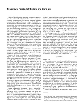
Summary Before data, we had no idea about Y, our“prior pdf” was fY(y) 1, 0 y 1. After seeing2 out of 2 people sampled have D, we updateto the “posterior pdf” fY(y 1,1) 3y2, 0 y 1.pdf3fY(y 1,1)1fY(y)0y136
Sect. 5.2 Expected Values(p. 197) For discrete RV‟s X, Y with joint pmf p, theexpected value of h(X,Y) isE[h( X , Y )] x y h( x, y) p( x, y)if finite.For continuous RV‟s X, Y with joint pdf f, theexpected value of h(X,Y) isE[h( X , Y )] h( x, y ) f ( x, y )dxdyif finite.37
Ex) X and Y have pdf f(x,y) x y, 0 x 1,0 y 1, and 0 else. Find E(XY2).1 1E ( XY ) xy ( x y )dxdy 17 / 72220 0(Check my integration) Extensions, by example: E[h( X , Y , Z )] h( x, y, z ) f ( x, y, z )dxdydz 38
Important Result:If X 1 , X 2 , , X n are independent RV' s, thenE[h1 ( X 1 )h2 ( X 2 ) hn ( X n )] E[h1 ( X 1 )]E[h2 ( X 2 )] E[hn ( X n )] “Under independence, the expectation of product product of expectations”Proof: (for n 2 in the continuous case.)39
E[h1 ( X 1 )h2 ( X 2 )] h ( x )h ( x ) f ( x , x )dx dx11221212 by indep. h ( x )h ( x ) f ( x ) f ( x )dx dx1122112212 h1 ( x1 ) f1 ( x1 )dx1 h2 ( x2 ) f 2 ( x2 )dx2 E[h1 ( X1 )]E[h2 ( X 2 )]40
Ex: X and Y have pdff ( x, y) (1 / 8) xe 0.50( x y), x 0, y 0and 0 elsewhere. Find E(Y/X). Note that f(x,y) “factors” (ranges on x,y are OK).Hence, X and Y are independent and 0.50 y 0.50xf ( x, y) [(.25) xe][(.50)e], x 0, y 0 f X ( x) f Y ( y ) 0.50( x y)Remark: If f ( x, y) cxethen X and Y are dependent,0 x y41
E(Y/X) E(Y) E(1/X) y(.50)e 0.50 y0 dy x (.25) xe 1 0.50 xdx (2)(.50) 10since, Y Exp(l .5) and mean of exponential is 1/l X has a Gamma pdf, but x(.25)xe 1 0.50 x0 dx (.25)(.5) /(.5)e 0.50 xdx0 .25 / .50 .5042
Important Concepts in Prob & Stat (p. 198)1. Covariance of X and Y Cov(X,Y) XYCov( X , Y ) E[( X m X )(Y mY )]Fact: Cov( X , Y ) E ( XY ) m X mYPoint: Cov(X,Y) measures dependence between X & Y If X and Y are independent, then Cov(X,Y) 0.Why: E(XY) E(X)E(Y) mX mY(indep. implies E(product) product(E‟s) ) But Cov(X,Y) 0 does not imply independence.43
IntuitionWe observe and graph many pairs of (X,Y).Suppose we gety‟sE(Y)Then (X-E(X)) andE(X)(Y-E(Y)) tend to havethe same sign, so the averageof their product (i.e., covariance) is positive.x‟s44
cov(X,Y) 0 cov(X,Y) 0(Not indep)cov(X,Y) 0 (& indep)45
2. Correlation between X and Y Corr(X,Y) XY Cov( X , Y ) X Y XYTheorem: 1 XY 1Point: XY measures dependence between X & Y in afashion that does not depend on units of measurements Sign of XY indicates direction of relationship Magnitude of XY indicates the strength of thelinear relationship between X and Y .5 .9
Results for Linear Combinations of RV‟s1. Recall: V (aX b) a 2 X2 S.D.(aX b) a X2. Extensions:Cov(aX b, cY d ) acCov( X , Y )Hence, Corr(aX b, cY d ) Corr( X , Y )V ( X Y ) V ( X ) V (Y ) 2Cov( X , Y )So, if X & Y are indep., V ( X Y ) V ( X ) V (Y )Thm : If X 1 , X 2 , , X n are indep.,V( X 1 X 2 X n ) V( X 1 ) V ( X 2 ) V ( X n )“Var( sum of indep. RV) sum ( their variances)”47
Ex) Pistons in CylindersLet X1 diameter of cylinder, X2 diameter ofpiston. “Clearance” Y 0.50 ( X1 – X2 ). AssumeX1 and X2 are independent andm1 80.95 cm, 1 .03 cm;m2 80.85 cm, 2 .02 cmFind mean and SD of Y:48
[ Y 0.50 ( X1 – X2 ). m1 80.95 cm, 1 .03 cm;m2 80.85 cm, 2 .02 cm ]1. mY E[.50 ( X1 – X2)] .50 [m1 – m2 ] .05 cm2. S.D.: Find V(Y), then square root(there‟s no general shortcut)V(Y) V[.50 ( X1 – X2 ) ] (.5)2 V( X1 – X2 ) .25 [(.03)2 (.02)2] 3.24 x 10 4so Y .018 cm (not .5 (.03 .02) .025)49
Ex), Cont‟dIf Y is too small, the piston can‟t move freely; ifY is too big, the piston isn‟t tight enough tocombust efficiently. Designers say a pistoncylinder pair will work if .01 Y .09.Assuming Y has a normal dist., findP(.01 Y .09).09 .05 .01 .05P(.01 Y .09) P Z .018 .018 P( 2.22 Z 2.22) .973650
FYI (not HW or Exams)If the normality assumption can‟t be claimed, youcan get a bound: P(.01 Y .09) P(.01 - .05 Y - .05 .09 - .05) P( Y - .05 .04) P( Y – mY .04) Chebyshev‟s Inequality: For any constant k 0,P( X – m k ) 1 – k-2 Set .04 k , so k-2 (.018 / .04)2Y Conclusion:P(.01 Y .09) P( Y - .05 .04) .797no matter what the dist of Y is !!!!51
FYI (not for HW or Exam): Conditional ExpectationRecall: X,Y have pdf f(x,y). ThenfX Y(x y) f(x,y)/fY(y) andP( X A Y y) f X Y ( x y)dxA(p. 156) Conditional expectation of h(X) given Y yDiscrete E[h( X ) y] h( x) p ( x y)xX Y Contin.E[h( X ) y ] h( x) f X Y ( x y )dx if they exist.52
Special cases (Contin. case; discrete are similar)1. Conditional mean of X given Y y ism X y xf X Y ( x y )dx 2. Conditional variance of X given Y y is 2X y E[( X m X y ) y] E ( X y) m222X yTry not to let all this notation fox you. Alldefinitions are the same, the conditioning just tellsus what PD or pdf to use.53
X and Y have pdff ( x, y) l e2Find 1. Need2X y ly,0 x yf X Y ( x y) f ( x, y) / fY ( y)yfY ( y ) l2 e ly dx l2 e ly y, y 00so2 lylef X Y ( x y ) 1 / y,0 x y2 lyyl e54
y2. Findm X y x(1 / y )dx 0.50 y0yE ( X y ) x (1 / y )dx y / 322203. So 2X y y / 3 ( y / 2) y / 1222255
Sec 5.3 - 5.4Last material for this courseLead-in to statistical inference: drawing conclusions aboutpopulation based on sample data we state our inferences and judge their value:based on probability56
Key Definitions and NotionsA. Target of Statistical Inference:1. Population: Collection of units or objects ofinterest.2. Pop Random Variable (RV): Numerical value Xassociated with each unit.3. Pop Dist.: Dist. of X over the pop.4. Parameters: Numerical summaries of pop.(mean, variance, proportion, )57
B. Inputs to Statistical Inference1.2.Sample: Subset of the populationSample Data: X1 , X2 , , Xn for the n units insample3. Statistic: Function of the datanMain ex) “sample mean” X Xi n i 14.Sampling variability: Different samples givedifferent values of a statistic. That is,Statistics are RV‟s5.Sampling distribution: Probability distribution ofa statistic.58
IdeaSample 1 X‟sgive Stat1Sample 2 X‟sgive Stat2PopulationSampling DistStat59
Key Point: Sampling Design Form of sampling dist. depends on how wepick samples In most cases, we want samples to berepresentative of pop.(i.e., not biased or special in some way).If X1 , X2 , , Xn are independent and identicallydistributed (i.i.d.), each having the pop. dist., theyform a random sample from the population Finding sampling dist:(1) Simulation and (2) Prob. theory results60
RemarkAlternative notion of representative samples:Simple random sample (SRS):Sample of n units chosen in a way that all samplesof n units have equal chance of being chosen Sampling without replacement: observations aredependent. When sampling from huge populations, SRS areapproximately Random Samples61
Sampling dist. via grunt workX the result of the roll of a fair diex:123456p(x):1/6 1/6 1/6 1/6 1/6 1/61 23 4 5 6X1, X2 be results of 2 indep. rolls. Dist of X :x : 1 1.5 2 2.5 3 3.5 4 4.5 5 5.5 6p(x ) : 1/36 2/36 3/36 4/36 5/36 6/36 5/36 4/36 3/36 2/36 533.53.5444.54.5563.5 44 4.54.555 5.55.5 612345 6
Simulation: Fundamental in modern applicationsMath/Stat has developed numerical methods to“generate” realizations of RV‟s from specified dist. Select a dist. and a statistic Simulate many random samples Compute statistic for each Examine the dist of the simulated statistics:histograms, estimates of their density, etc.63
Simple Ex) Pop. Dist: X N(10, 4). Statistic X Draw k 1000 random samples (in practice, usemuch larger k); compute means and make histogramsfor four different sample sizes
n 10, k 50,000
Various nn 20n 30n 5n 10
Various nn 20n 30n 5n 10
WeibullLognormal
Last Time1.Population: Collection of objects of interest.2.Population RV: X (value for each object in pop.)3.Population Dist.: Dist. of RV X over the pop.4.Parameters: Numerical summaries of pop. (ex. m, 5.Sample: Subset of the population6.Data: X1 , X2 , , Xn for the objects in sample7.Statistic: Function of the dataKey: Sampling variability: different samples give differentvalues of a statistic. Statistics are RV’s8.Sampling distribution: Distribution of a statistic.Key: Distribution of statistic depends on how sample istaken71
Sampling DesignIn most cases, we want samples to be representativeof pop. (i.e., not biased or special in some way).In this course (and most applications):If X1 , X2 , , Xn are independent and identicallydistributed (i.i.d.), each having the pop. dist., theyform a random sample from the population Finding sampling dist:(1) Simulation (last time)(2) Prob. theory results (today)72
RemarkAlternative notion of representative samples:Simple random sample (SRS):Sample of n units chosen in a way that all samplesof n units have equal chance of being chosen Sampling without replacement: observations aredependent. When sampling from huge populations, SRS areapproximately Random Samples73
Main Statistics (Sect. 5.4; p. 229-230)n1. Sample Mean:or “X-bar”X Xi 1inn2. Sample Variance:or “S-squared”S2 (Xi 1i X)2n 13. Sample proportion: example later74
Sect. 5.4: Dist. of X-barProposition (p. 213):If X1 , X2 , , Xn is a (iid) random samplefrom a population distribution with mean m andvariance 2, then1. mX 2. 2Xdef defE( X ) mV (X ) 2nand X n75
Proof: n 1. E ( X ) E X i / n i 1 n 1 E( X i ) n i 1 nm mnConstants comeoutside exp‟ andE(sum) sum(E‟s)76
n 2. var( X ) var X i / n i 1 n 1 2 var( X i ) n i 1 22n 2 nnConstants comeout of Varsquared andfor indep RV,V(sum) sum(V‟s)77
Remarks:1. In statistics, we typically use X to estimate m andS2 to estimate 2.When E(Estimator) target , we say the estimator isunbiased(note: S is not unbiased for )2. Independence of the Xi„s is only needed for thenvariance result.3. Results stated for sum‟s: Let T0 X ii 1Under the assumptions of the Proposition,E (T0 ) nm , V (T0 ) n 2and T0 n 78
More resultsProposition (p. 214): If X1 , X2 , , Xn is an iidrandom sample from a population having a normaldistribution with mean m and variance 2, thenX has a normal distribution with mean m andvariance 2 /nThat is,2X N (m , n)Proof: Beyond our scope (not really hard, just usesfacts text doesn‟t cover)79
Large sample (large n) properties of X-barAssume X1 , X2 , , Xn are a random sample (iid)from a population with mean m and variance 2 .(normality is not assumed)1. Law of Large NumbersRecall that m X m and note thatn 2X 2n 0We can prove that with probability 1,n X m81
2. Central Limit Theorem (CLT) (p. 215)Under the above assumptions (iid random sample)X m D Z N (0,1) n“converges in dist. to”or “has limiting dist.”Point: For n large,X N (m , n)2“approx dist as”So for n large, we can approx prob‟s for X-bar eventhough we don‟t know the pop. dist.83
2. Central Limit Theorem (CLT) For SumsUnder the above assumptions (iid random sample)T0 nm D Z N (0,1) nPoint: For n large,T0 N (nm , n )2So for n large, we can approx prob‟s for T0 eventhough we don‟t know the pop. dist.84
Last Time:nDist. of “X-bar”: X Xnii 1Three Main Results: Assumption common to all:X1 , X2 , , Xn is a (iid) random sample froma pop. dist. with mean m and variance 2. 1. mX m and n2X22. If the pop. dist. is normal, thenX N (m , n)23. If n is largeX N (m , n)285
Restate for the sum:T0 i 1 X in1. mT0 nm and n 2T022. If the pop. dist. is normal, thenT0 N (nm , n )2(Theorem: sum of indep. normals is normal)3. If n is largeT0 N (nm , n )286
Ex) Estimate the average height of men in somepopulation. Assume pop. is 2.5 in. We willcollect an iid sample of 100 men. Find the prob. thattheir sample mean will be within .5 in of the pop. mean. Let m be the population mean. FindP( X m .5) 2 2.52 2.52 Applying CLT, X N m , 2 n100 10 soP( X m .5) P( Z .5 / .25) P( Z 2) .95
Ex) Application for “sums”: Binomial Dist.1. Recall (p. 88): A Bernoulli RV X takes on values 1or 0. Set P(X 1) p . Easy to check thatmX p and X2 p(1 p)2. X Bin( n, p ) is the sum of n iid Bernoulli‟s.22Applying result mT0 nm and T0 n givesm X np and 2X np(1 p)3. CLT: For n large,X N (np, np(1 p))Remark: CLT doesn‟t include “continuity correction”
Ex) Continued. In practice, we may not know p1. Traditional estimator: sample proportion, p-hatpˆ X n2. Key: since X Bin( n, p ) is the sum of n iidBernoulli‟s, p-hat is a sample meani.e., let Bi , i 1, , n denote the Bernoulli‟s:pˆ X n i 1 Bi nn3. Apply CLT: For n large,p(1 p) ˆ N p,p n
Ex) Service times for checkout at a store are indep.,average 1.5 min., and have variance 1.0 min2. Findprob. 100 customers are served in less than 2 hours. Let Xi service time of ith customer.n Service time for 100 customers: T Xii 1 Applying the CLT, T N (nm 100(1.5), n 2 100(1)) So, T 150 120 150 P(T 120) P 10 10 P( Z 3) .0013
Ex) Common Class of Applications In many cases, we know the distribution of the sumof independent RV‟s, but if that dist. is complicated,we may still want to use CLT approximations. Example:1) Theorem. If X1 Poi(l1) , , Xk Poi(lk) areindep. Poisson RV‟s, thenT i 1 X i Poi (lT i 1 li )kk(i.e., “sum of indep. Poissons is Poisson”)Proof: not hard, but beyond the text
2) Implication: Suppose Y Poi(l) where l is very2large. Recall mY l and Y l3) Slick Trick: pretend Y sum of n iid Poisson‟s,each with parameter l* where l nl* and n islarge. That is, Xi Poi(l*) for i 1, , n.By the Theorem:nni 1i 1Y X i Poi (l l* nl*)4) Apply CLT:Y ll N (0,1)
Ex) Number of flaws in a unit of material has aPoisson dist. with mean 2. We receive a shipment of50 units.a) Find prob that the total number of flaws in the 50units is less than 110.b) Find prob that at least 20 of the 50 have morethan 2 flaws.c) Find prob that at least 2 of the 50 have more than6 flaws.In the following solutions, we assume the number offlaws in the 50 units are independent RV‟s
Find prob that the total number of flaws in the 50units is less than 110. Since sum of indep Poisson‟s is Poisson:T total number of flaws is Poi( l 2(50) 100)Since l 100 is large, use normal approx.: T 100 110 100 P(T 110) P 10 10 P( Z 1) .8413Note, with cont. correction,109.5 100 P(T 110) P Z .828910 (“Exact” Poisson calculation: .8294)
b) Find prob that at least 20 of the 50 have morethan 2 flaws. Let X number units with more than 2 flaws.Since the units are indep., X is Bin(n 50, p) where p P(Y 2) where Y is Poi( l 2). Using Poisson pmf, check that p .3233 Apply Normal approx. to binomial:2 m X np 50(.3233) 16.165X np(1 p) 10.94so P( X 20) P(Z (20 16.165)or, with cont. correctionP( X 20) P(Z (19.5 16.165)(Exact Binomial: .1566)10.94 ) .12310.94 ) .1562
c) Find prob that at least 2 of the 50 have more than6 flaws. Now, X Bin(50, p) where p P(Y 6) and Y Poi( l 2). Poisson pmf gives p .0045 Hence, np 50(.0045) .225 which is way toosmall for normal approx. Use Poisson approx to Bin:P(X 2) 1 – P( X 1) 1-P(X 0,1)Using Poi( l .225), we getexp(-.225) (1.225) .023(Exact Binomial: .0215)
CLT: Assume X1 , X2 , , Xn is a (iid) randomsample from a distribution with mean m and22variance . If n is large, X N ( m , n)2and the sum T0 N (nm , n )Note: In practice, we may need to estimate 2. Typicalprocedure: input the sample variance. Theorem:nn S 2 ( X i X ) 2 (n 1) 2 with prob 1i 1Remark: Rule of Thumb (p. 217) “If n 30, CLT can beused” is nonsense. This is only OK if the pop dist isreasonably symmetric.(Also p. 217, text says use CLT approx. to bin. if np 10, soif p .10 and n 50, np 5 so don‟t use CLT(though n 30))97
Two important settings/applicationsA. Sample Size Determination.Estimate the unknown mean m of some distribution.Basic procedure:i. Choose a random sample (iid) of n observations.ii. Use their sample mean X to estimate mIdea: we know accuracy of estimate increases as ndoes, but so does cost of data collection.
How large should n be to obtain a desired accuracy?Quantification: For specified choices of M and a,choose n large enough thatP( X m M ) 1 a M is the margin of error a is the error rate; a small (.05 is a common choice)
Apply CLT: for n large,P( X m M ) P( Z M / n) 1 aConclusion:M2 1.96soweneedn (1.96 /M)a .05: / nM2a .01: 2.576 so we need n (2.576 / M ) / n
Notes1. Of course, round up to an integer.2. Procedure requires a guess at 3. Analysis is valid for all n if the population isnormal.4. Otherwise, if the answer turns out to be small,CLT does not apply, so analysis failed(Remark: you could use Chebyshev‟s Inequality, moreconservative, but works for all distributions and all n)
Ex) Assess accuracy of lab scale. Weigh a sampleknown to weigh 100 gm repeatedly and estimate themean m 100 b where b (gm) denotes the scale‟sbias. Assume s 10 gm. Find n so that we estimate bwith M 1 and a .05. (Note: bˆ X 100 )P( bˆ b M ) 1 aM 1.96 so n (1.96 10 / 1) 2 385 / nNote: Decimal points of accuracy can be expensiveMa .05a .0110.10.0138538,4163,841,60066466,3586,635,776
Apply to Estimating a Pop. ProportionUnknown proportion p typically estimated by sampleproportion: pˆ X / nCLT: For large n, the sample proportion, p(1 p) pˆ N p, n For fixed M, how large should n be so thatP( pˆ p M ) P( Z Mp(1 p) / n) 1 aNote: we need a guess, say p*, of p. Approaches:1. Based on past data and other information.2. Choosing p* .5 is conservative.103
Example results: a .05 and p* 0.50MP( Z ) .95.50(.50) / nMgives.025M 2,.02.5(1 .5) / n.012so n 1 / M.005 nM in %16002.5%25002.0%10,0001.0%250,0000.50%This is why “statistics” works: increasing n from 10,000 to250,000 reduces the M very little.If samples aren‟t representative, even millions ofobservations may be useless or misleading.104
B. Simulation --- Monte Carlo1. Suppose X f(x) (stated for cont. RV, but appliesto discrete RV‟s too). We need E(h(X)) for somefunction h, but the calculation is very difficult.i. Simulate X1 , X2 , , Xn iid f(x)ii. Compute h(X1), h(X2), , h(Xn) and findh i 1 h( X i ) / nniii. CLT: for n large,h N ( E (h( X )), 2hn)
iv. We need to estimate n22Most use sh (h( X i ) h ) /( n 1) 2hi 1Recall: n S h2 h2 with prob 1v. We can apply the sample size calculations above tochoose n to control accuracy.
2. Suppose X f(x) 0, for 0 x 1, but it is hard tosimulate from f. Recall that1E ( h( X )) h( x) f ( x) dx0Note: if Y Uniform(0,1) [i.e, pdf 1 on (0,1)]1E (h( X )) h( y ) f ( y )dy E (h(Y ) f (Y ))0i. Simulate Y1 , Y2 , , Yn iid Uniform(0,1)ii. Compute h(Y1)f(Y1), h(Y2)f(Y2), , h(Yn)f(Yn)nand findhf i 1 h( X i ) f ( X i ) / n
iii. CLT: for n large,hf N ( E (h( X )), 2hfn)Proceed as above3. Numerical integration. Estimate the integral1I h( x) dx0Note that I E (h( X )) where X Uniform(0,1)i. Simulate X1 , X2 , , Xn iid Uniform(0,1)ii. Compute h(X1), h(X2), , h(Xn) and findnˆI h i 1 h( X i ) / nand proceed as above
Remarks1. Monte Carlo integrationi. Purely deterministic problem approached viaprobabilistic methods.ii. Real value: Estimating high dimensionalintegrals2. I‟ve just scratched the surface of applications ofMonte Carlo.3. Key: We obtain estimates and probabilistic errorbounds. When simulation is cheap, we can makethese errors arbitrarily small with very high prob.
the integral of its pdf over A: no conditional; use the marginal pdf with a condition; use the right cond‟l pdf Interpretation: For cont. X, P(X x) 0, so by Chap 2 rules, is meaningless. -There is a lot of theory that makes sense of this -For our purposes, think of it as an approximation to