Transcription
STATISTICSPROBABILITY ANDSTATISTICSSESSION 7STATISTICSSESSION 7
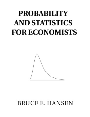
SESSION 7Probability and StatisticsProbability LineProbability is the chance that something will happen. It can be shown on a line.The probability of an event occurring is somewhere between impossible and certain.As well as words we can use numbers (such as fractions or decimals) to show the probability ofsomething happening: Impossible is zeroCertain is one.Here are some fractions on the probability line:We can also show the chance that something will happen:a) The sun will rise tomorrow.b) I will not have to learn mathematics at school.c) If I flip a coin it will land heads up.d) Choosing a red ball from a sack with 1 red ball and 3 green balls
Between 0 and 1 The probability of an event will not be less than 0.This is because 0 is impossible (sure that something will not happen).The probability of an event will not be more than 1.This is because 1 is certain that something will happen.Calculation and ChanceMost experimental searches for paranormal phenomena are statistical in nature. A subjectrepeatedly attempts a task with a known probability of success due to chance, then the number ofactual successes is compared to the chance expectation. If a subject scores consistently higher orlower than the chance expectation after a large number of attempts, one can calculate theprobability of such a score due purely to chance, and then argue, if the chance probability issufficiently small, that the results are evidence for the existence of some mechanism(precognition, telepathy, psychokinesis, cheating, etc.) which allowed the subject to performbetter than chance would seem to permit.Suppose you ask a subject to guess, before it is flipped, whether a coin will land with heads ortails up. Assuming the coin is fair (has the same probability of heads and tails), the chance ofguessing correctly is 50%, so you'd expect half the guesses to be correct and half to be wrong.So, if we ask the subject to guess heads or tails for each of 100 coin flips, we'd expect about 50of the guesses to be correct. Suppose a new subject walks into the lab and manages to guessheads or tails correctly for 60 out of 100 tosses. Evidence of precognition, or perhaps thesubject's possessing a telekinetic power which causes the coin to land with the guessed face up?Well, no. In all likelihood, we've observed nothing more than good luck. The probability of 60correct guesses out of 100 is about 2.8%, which means that if we do a large number ofexperiments flipping 100 coins, about every 35 experiments we can expect a score of 60 orbetter, purely due to chance.But suppose this subject continues to guess about 60 right out of a hundred, so that after ten runsof 100 tosses—1000 tosses in all, the subject has made 600 correct guesses. The probability of
that happening purely by chance is less than one in seven billion, so it's time to start thinkingabout explanations other than luck. Still, improbable things happen all the time: if you hit a golfball, the odds it will land on a given blade of grass are millions to one, yet (unless it ends up inthe lake or a sand trap) it is certain to land on some blades of grass.Finally, suppose this “dream subject” continues to guess 60% of the flips correctly, observed bymultiple video cameras, under conditions prescribed by skeptics and debunkers, using a coinprovided and flipped by The Amazing Randi himself, with a final tally of 1200 correct guesses in2000 flips. You'd have to try the 2000 flips more than 5 1018 times before you'd expect thatresult to occur by chance. If it takes a day to do 2000 guesses and coin flips, it would take morethan 1.3 1016 years of 2000 flips per day before you'd expect to see 1200 correct guesses due tochance. That's more than a million times the age of the universe, so you'd better get started soon!Claims of evidence for the paranormal are usually based upon statistics which diverge so farfrom the expectation due to chance that some other mechanism seems necessary to explain theexperimental results. To interpret the results of our RetroPsychoKinesis experiments, we'll beusing the mathematics of probability and statistics, so it's worth spending some time explaininghow we go about quantifying the consequences of chance.Note to mathematicians: The following discussion of probability is deliberately simplified to consider onlybinomial and normal distributions with a probability of 0.5, the presumed probability of success in the experimentsin question. I decided that presenting and discussing the equations for arbitrary probability would only decrease theprobability that readers would persevere and arrive at an understanding of the fundamentals of probability theory.Twelve and a half cents: one bit!In slang harking back to the days of gold doubloons and pieces of eight, the United Statesquarter-dollar coin is nicknamed “two bits”. The Fourmilab radioactive random numbergenerator produces a stream of binary ones and zeroes, or bits. Since we expect the generator toproduce ones and zeroes with equal probability, each bit from the generator is equivalent to acoin flip: heads for one and tails for zero. When we run experiments with the generator, in effect,we're flipping a binary coin, one bit—twelve and a half cents!Two BitsHeadsOne BitTailsHeadsTails(We could, of course, have called zero heads and one tails; since both occur with equalprobability, the choice is arbitrary.) Each bit produced by the random number generator is a flip
of our one-bit coin. Now the key thing to keep in mind about a genuine random numbergenerator or flip of a fair coin is that it has no memory or, as mathematicians say, each bit fromthe generator or flip is independent. Even if, by chance, the coin has come up heads ten times ina row, the probability of getting heads or tails on the next flip is precisely equal. Gamblerswho've seen a coin come up heads ten times in a row may believe “tails is way overdue”, but thecoin doesn't know and couldn't care less about the last ten flips; the next flip is just as likely to bethe eleventh head in a row as the tail that breaks the streak.Even though there is no way whatsoever to predict the outcome of the next flip, if we flip a coina number of times, the laws of probability allow us to predict, with greater accuracy as thenumber of flips increases, the probability of obtaining various results. In the discussion thatfollows, we'll ignore the order of the flips and only count how many times the coin came upheads. Since heads is one and tails is zero, we can just add up the results from the flips, or thebits from the random generator.Four FlipsSuppose we flip a coin four times. Since each flip can come up heads or tails, there are 16possible outcomes, tabulated below, grouped by the number of heads in the four flips.Numberof HeadsResults of FlipsNumberof Ways011426
3441Number of Ways summarises how many different ways the results of the four flips could end upwith a given number of heads. Since the only way to get zero heads is for all four flips to be tails,there's only one way that can occur. One head out of four flips can happen four different wayssince each of the four flips could have been the head. Two heads out of four flips can happen sixdifferent ways, as tabulated. And since what's true of heads applies equally to tails, there are fourways to get three heads and one way to get four.Mathematically, the number of ways to get x heads (or tails) in n flips is spoken of as the“number of combinations of n things taken x at a time”, which is written as:This, it turns out, can be calculated for any positive integers n and x whatsoever, as follows.For example, if we plug in 4 for n and 2 for x, we get4! / (2! (4 2)!) 4! / (2! 2!) 24 / (2 2) 24 / 4 6as expected. Plotting the number of ways we can get different numbers of heads yields thefollowing graph.
ProbabilitySince the coin is fair, each flip has an equal chance of coming up heads or tails, so all 16 possibleoutcomes tabulated above are equally probable. But since there are 6 ways to get 2 heads, in fourflips the probability of two heads is greater than that of any other result. We express probabilityas a number between 0 and 1. A probability of zero is a result which cannot ever occur: theprobability of getting five heads in four flips is zero. A probability of one represents certainty: ifyou flip a coin, the probability you'll get heads or tails is one (assuming it can't land on the rim,fall into a black hole, or some such).The probability of getting a given number of heads from four flips is, then, simply the number ofways that number of heads can occur, divided by the number of total results of four flips, 16. Wecan then tabulate the probabilities as follows.Number Numberof Heads of WaysProbability011/16 0.0625144/16 0.25266/16 0.375344/16 0.25411/16 0.0625Since we are absolutely certain the number of heads we get in four flips is going to be betweenzero and four, the probabilities of the different numbers of heads should add up to 1. Summingthe probabilities in the table confirms this. Further, we can calculate the probability of anycollection of results by adding the individual probabilities of each. Suppose we'd like to knowthe probability of getting fewer than three heads from four flips. There are three ways this canhappen: zero, one, or two heads. The probability of fewer than three, then, is the sum of the
probabilities of these results, 1/16 4/16 6/16 11/16 0.6875, or a little more than two outof three. So to calculate the probability of one outcome or another, sum the probabilities.To get probability of one result and another from two separate experiments, multiply theindividual probabilities. The probability of getting one head in four flips is 4/16 1/4 0.25.What's the probability of getting one head in each of two successive sets of four flips? Well, it'sjust 1/4 1/4 1/16 0.0625.The probability for any number of heads x in any number of flips n is thus:the number of ways in which x heads can occur in n flips, divided by the number of differentpossible results of the series of flips, measured by number of heads. But there's no need to sumthe combinations in the denominator, since the number of possible results is simply two raised tothe power of the number of flips. So, we can simplify the expression for the probability to:More FlipsLet's see how the probability behaves as we make more and more flips. Since we have a generalformula for calculating the probability for any number of heads in any number of flips, we cangraph of the probability for various numbers of flips.
8 Flips16 Flips32 Flips
64 Flips128 FlipsIn every case, the peak probability is at half the number of flips and declines on both sides, moresteeply as the number of flips increases. This is the simple consequence of there being manymore possible ways for results close to half heads and tails to occur than ways that result in asubstantial majority of heads or tails. The RPKP experiments involve a sequence of 1024 randombits, in which the most probable results form a narrow curve centred at 512. A document givingprobabilities for results of 1024 bit experiments with chance expectations greater than one in 100thousand million runs is available, as is a much larger table listing probabilities for all possibleresults. (The latter document is more than 150K bytes and will take a while to download, andcontains a very large table which some Web browsers, particularly on machines with limitedmemory, may not display properly.)Perfectly NormalAs we make more and more flips, the graph of the probability of a given number of headsbecomes smoother and approaches the “bell curve”, or normal distribution, as a limit. Thenormal distribution gives the probability for x heads in n flips as:
where μ n/2 and σ is the standard deviation, a measure of the breadth of the curve which, forequal probability coin flipping, is:We keep the standard deviation separate, as opposed to merging it into the normal distributionprobability equation, because it will play an important rôle in interpreting the results of ourexperiments. To show how closely the probability chart approaches the normal distribution evenfor a relatively small number of flips, here's the normal distribution plotted in red, with the actualprobabilities for number of heads in 128 flips shown as blue bars.The probability the outcome of an experiment with a sufficiently large number of trials is due tochance can be calculated directly from the result, and the mean and standard deviation for thenumber of trials in the experiment. For additional details, including an interactive probabilitycalculator, please visit the z Score Probability Calculator.Calculation and RealityThis is all very persuasive, you might say, and the formulas are suitably intimidating, but doesthe real world actually behave this way? Well, as a matter of fact, it does, as we can see from asimple experiment. Get a coin, flip it 32 times, and write down the number of times heads cameup. Now repeat the experiment fifty thousand times. When you're done, make a graph of thenumber of 32-flip sets which resulted in a given number of heads. Hmmmm 32 times 50,000 is1.6 million, so if you flip the coin once a second, twenty-four hours per day, it'll take eighteenand a half days to complete the experiment .
Instead of marathon coin-flipping, let's use the same HotBits hardware random number generatorour experiments employ. It's a simple matter of programming to withdraw 1.6 million bits fromthe generator, divide them up into 50,000 sets of 32 bits each, then compute a histogram of thenumber of sets containing each possible number of one bits (heads). The results from thisexperiment are presented in the following graph.The red curve is the number of runs expected to result in each value of heads, which is simplythe probability of that number of heads multiplied by the total number of experimental runs,50,000. The blue diamonds are the actual number of 32 bit sets observed to contain each numberof one bits. It is evident that the experimental results closely match the expectation fromprobability. Just as the probability curve approaches the normal distribution for large numbers ofruns, experimental results from a truly random source will inexorably converge on thepredictions of probability as the number of runs increases.If your Web browser supports Java applets, ourProbability Pipe Organ lets you run interactiveexperiments which demonstrate how the results fromrandom data approach the normal curve expectation asthenumberofexperimentsgrowslarge.Experiments and Expectations
Performing an experiment amounts to asking the Universe a question. For the answer, theexperimental results, to be of any use, you have to be absolutely sure you've phrased the questioncorrectly. When searching for elusive effects among a sea of random events by statistical means,whether in particle physics or parapsychology, one must take care to apply statistics properly tothe events being studied. Misinterpreting genuine experimental results yields errors just asserious as those due to faults in the design of the experiment.Evidence for the existence of a phenomenon must be significant, persistent, and consistent.Statistical analysis can never entirely rule out the possibility that the results of an experimentwere entirely due to chance—it can only calculate the probability of occurrence by chance. Onlyas more and more experiments are performed, which reproduce the supposed effect and, bydoing so, further decrease the probability of chance, does the evidence for the effect becomepersuasive.To show how essential it is to ask the right question, consider an experiment in which the subjectattempts to influence a device which generates random digits from 0 to 9 so that more nines aregenerated than expected by chance. Each experiment involves generation of one thousandrandom digits. We run the first experiment and get the following 2159232The digit frequencies from this run are:Digit Occurrences0941812963111
4845111611171128919109There's no obvious evidence for a significant excess of nines here (we'll see how to calculate thisnumerically before long). There was an excess of nines over the chance expectation, 100, butgreater excesses occurred for the digits 3, 5, 6, and 7. But take a look at the first line of 65786865762.These digits were supposed to be random, yet in the first thousand, the first dozen for that matter,we found a pattern as striking as “999999”. What's the probability of that happening? Just thenumber of possible numbers of d digits which contain one or more sequences of p or moreconsecutive nines:Plugging in 1000 for d and 6 for p yields:So the probability of finding “999999” in a set of 1000 random digits is less than one in athousand! So then, are the digits not random, after all? Might our subject, while failing toinfluence the outcome of the experiment in the way we've requested, have somehow marked theresults with a signature of a thousand-to-one probability of appearing by chance? Or have wesimply asked the wrong question and gotten a perfectly accurate answer that doesn't mean whatwe think it does at first glance?The latter turns out to be the case. The data are right before our eyes, and the probability wecalculated is correct, but we asked the wrong question, and in doing so fell into a trap litteredwith the bones of many a naïve researcher. Note the order in which we did things. We ran theexperiment, examined the data, found something seemingly odd in it, then calculated theprobability of that particular oddity appearing by chance. We asked the question, “What is the
probability of ‘999999’ appearing in a 1000 digit random sequence?” and got the answer “lessthan one in a thousand”, a result most people would consider significant. But since we calculatedthe probability after seeing the data, in fact we were asking the question “What is the chance that‘999999’ appears in a 1000 digit random sequence which contains one occurrence of‘999999’?”. The answer to that question is, of course, “certainty”.In the original examination of the data, we were really asking “What is the probability we'll findsome striking sequence of six digits in a random 1000 digit number?”. We can't preciselyquantify that without defining what “striking” means to the observer, but it is clearly quite high.Consider that I could have made the case just as strongly for “000000”, “777777” or any othersix-digit repeat. That alone reduces the probability of occurrence by chance to one in ten. Or,perhaps I might have pointed out a run of digits like “123456”, “012345”, “987654”, and so on;or the first five or six digits of a mathematical constant such as Pi, e, or the square root of two;regular patterns like “101010”, “123321”, or a multitude of others; or maybe my telephone orlicense plate number, or the subject's! It is, in fact, very likely you'll find some pattern youconsider striking in a random 1000-digit number.But, of course, if you don't examine the data from an experiment, how are you going to notice ifthere's something odd about it? Now we'll see how a hypothesis is framed, tested by a series ofexperiments, and confirmed or rejected by statistical analysis of the results. So, let's pursue this abit further, exploring how we frame a hypothesis based on an observation, run experiments totest it, and then analyse the results to determine whether they confirm or deny the hypothesis,and to what degree of certainty.Our observation, based on examining the first thousand random digits, is that “999999” appearsonce, while the probability of “999999” appearing in a randomly chosen 1000 digit number isless than one in a thousand. Based on this observation we then suggest:Hypothesis: The sequence “999999” appears more frequently in 1000-digit sequences with thesubject attempting to influence the generator than would be expected by chance.We can now proceed to test this experimentally. If the sequence “999999” has a probability ofoccurring in a 1000 digit sequence of 0.000995, then for a thousand consecutive 1000 digitsequences (a million digits in all), the probability of “999999” appearing will be 0.995, almostunity. (To be correct, it's important to test each 1000 digit sequence separately, then sum the results for 1000consecutive sequences. If we were to scan all million digits as one sequence, we would count cases where thesequence “999999” begins in one 1000 digit sequence and ends in the next. The probability (which you can calculatefrom the equation above) of finding “999999” in a million digit sequence is 0.999995, somewhat higher than the0.995 with the million digits are treated as separate 1000 digit experiments.)We will perform, then, the following experiment. With our ever-patient subject continuing toattempt to influence the output of the generator, we will produce a million more sequences of1000 digits and, in each, count occurrences of “999999”. Every 1000 sequences, we'll record thenumber of occurrences, repeating the process until we've generated a thousand runs of a milliondigits—109 digits in all. With that data in hand, we'll see whether the “999999 effect” is genuineor a fluke attributable to chance.
Here is a plot of the number of occurrences of the sequence “999999” per block of 1000 digitsover the thousand repetitions of the thousand sequence experiment. The number of occurrencesexpected by chance, 0.995, is marked by the green line.At the outset, the results diverged substantially from chance, as is frequently the case for smallsample sizes. But as the number of experiments increased, the results converged toward thechance expectation, ending up in a decreasing magnitude random walk around it. This isprecisely what is expected from probability theory, and hence we conclude no “999999 effect”exists.Ensembles of Experiments: the X² (Chi-Square) TestSo far, we've seen how the laws of probability predict the outcome of large numbers ofexperiments involving random data, how to calculate the probability of a given experimentalresult being due to chance, and how one goes about framing a hypothesis, then designing andrunning a series of experiments to test it. Now it's time to examine how to analyse the resultsfrom the experiments to determine whether they provide evidence for the hypothesis and, if so,how much.Since its introduction in 1900 by Karl Peterson, the chi-square (X²) test has become the mostwidely used measure of the significance to which experimental results support or refute ahypothesis. Applicable to any experiment where discrete results can be measured, it is used inalmost every field of science. The chi-square test is the final step in a process which usuallyproceeds as follows.1. Based either on theory or examination of empirical data, a phenomenon is suggested toexist.2. A hypothesis is framed incorporating the supposed phenomenon.3. An experiment is designed to test the hypothesis. The experiment must produce resultswhich differ based on the validity of the hypothesis. The results of the experiment for the
hypothesis-false (null hypothesis) case are calculated and, if appropriate, verified by acontrol experiment in which the hypothesised effect is excluded.4. A series of experiments are conducted, and the results tabulated.5. The chi-square test is applied to determine the significance of the discrepancy betweenthe calculated null hypothesis case and the experimental results, and the probability thatthe discrepancy is the result of chance. If that probability is very low, the experimentprovides evidence for the hypothesis.No experiment or series of experiments can ever prove a hypothesis; one can only rule out otherhypotheses and provide evidence that assuming the truth of the hypothesis better explains theexperimental results than discarding it. In many fields of science, the task of estimating the nullhypothesis results can be formidable, and can lead to prolonged and intricate arguments aboutthe assumptions involved. Experiments must be carefully designed to exclude selection effectswhich might bias the data.Fortunately, retropsychokinesis experiments have an easily stated and readily calculated nullhypothesis: “The results will obey the statistics for a sequence of random bits.” The fact that thedata are prerecorded guarantees (assuming the experiment software is properly implemented andthe results are presented without selection or modification) that run selection or other forms ofcheating cannot occur. (Anybody can score better than chance at coin flipping if they're allowedto throw away experiments that come out poorly!) Finally, the availability of all the programs insource code form and the ability of others to repeat the experiments on their own premises willallow independent confirmation of the results obtained here.So, as the final step in analysing the results of a collection of n experiments, each with k possibleoutcomes, we apply the chi-square test to compare the actual results with the results expected bychance, which are just, for each outcome, its probability times the number of experiments n.Mathematically, the chi-square statistic for an experiment with k possible outcomes, performed ntimes, in which Y1, Y2, Yk are the number of experiments which resulted in each possibleoutcome, where the probabilities of each outcome are p1, p2, pk is:It's evident from examining this equation that the closer the measured values are to thoseexpected, the lower the chi-square sum will be. Further, from a chi-square sum, the probability Qthat the X² sum for an experiment with d degrees of freedom (where d k 1, one less the numberof possible outcomes) is consistent with the null hypothesis can be calculated as:
Where Γ is the generalisation of the factorial function to real and complex arguments:Unfortunately, there is no closed form solution for Q, so it must be evaluated numerically. Ifyour Web browser supports JavaScript, you can use the Chi-Square Calculator to calculate theprobability from a chi-square value and number of possible outcomes, or calculate the chi-squarefrom the probability and the number of possible outcomes.In applying the chi-square test, it's essential to understand that only very small probabilities ofthe null hypothesis are significant. If the probability that the null hypothesis can explain theexperimental results is above 1%, an experiment is generally not considered evidence of adifferent hypothesis. The chi-square test takes into account neither the number of experimentsperformed nor the probability distribution of the expected outcomes; it is valid only as thenumber of experiments becomes large, resulting in substantial numbers for the most probableresults. If a hypothesis is valid, the chi-square probability should converge on a small value asmore and more experiments are run.Now let's examine an example of how the chi-square test identifies experimental results whichsupport or refute a hypothesis. Our simulated experiment consists of 50,000 runs of 32 randombits each. The subject attempts to influence the random number generator to emit an excess ofone or zero bits compared to the chance expectation of equal numbers of zeroes and ones. Thefollowing table gives the result of a control run using the random number generator without thesubject's attempting to influence it. Even if the probability of various outcomes is easilycalculated, it's important to run control experiments to make sure there are no errors in theexperimental protocol or apparatus which might bias the results away from those expected. Thetable below gives, for each possible number of one bits, the number of runs which resulted inthat count, the expectation from probability, and the corresponding term in the chi-square sum.The chi-square sum for the experiment is given at the bottom.Control Run
Ones0Results0Expectation1.16 10 5X² Term1.16 10 231.74162
0.0003725293201.16 10 5X² Sum1.16 10 523.8872Entering the X² sum of 23.8872 and the degrees of freedom (32, one less than the 33 possibleoutcomes of the experiment) into the Chi-Square Calculator gives a
Probability and Statistics Probability Line Probability is the chance that something will happen. It can be shown on a line. The probability of an event occurring is somewhere between impossible and certain. As well as words we can use numbers (such as fractions or decimals) to show t