Transcription
Power laws, Pareto distributions and Zipf’s lawMany of the things that scientists measure have a typical size or “scale”—a typical value around which individual measurements are centred. A simple examplewould be the heights of human beings. Most adult human beings are about 180cm tall. There is some variationaround this figure, notably depending on sex, but wenever see people who are 10cm tall, or 500cm. To makethis observation more quantitative, one can plot a histogram of people’s heights, as I have done in Fig. 1a.The figure shows the heights in centimetres of adultmen in the United States measured between 1959 and1962, and indeed the distribution is relatively narrowand peaked around 180cm. Another telling observationis the ratio of the heights of the tallest and shortest people. The Guinness Book of Records claims the world’stallest and shortest adult men (both now dead) as having had heights 272cm and 57cm respectively, makingthe ratio 4.8. This is a relatively low value; as we will seein a moment, some other quantities have much higherratios of largest to smallest.Figure 1b shows another example of a quantity with atypical scale: the speeds in miles per hour of cars on themotorway. Again the histogram of speeds is stronglypeaked, in this case around 75mph.But not all things we measure are peaked around atypical value. Some vary over an enormous dynamicrange, sometimes many orders of magnitude. A classicexample of this type of behaviour is the sizes of townsand cities. The largest population of any city in the USis 8.00 million for New York City, as of the most recent(2000) census. The town with the smallest population isharder to pin down, since it depends on what you calla town. The author recalls in 1993 passing through thetown of Milliken, Oregon, population 4, which consistedof one large house occupied by the town’s entire humanpopulation, a wooden shack occupied by an extraordinary number of cats and a very impressive flea market.According to the Guinness Book, however, America’ssmallest town is Duffield, Virginia, with a population of52. Whichever way you look at it, the ratio of largestto smallest population is at least 150 000. Clearly this isquite different from what we saw for heights of people.And an even more startling pattern is revealed whenwe look at the histogram of the sizes of cities, which isshown in Fig. 2.In the left panel of the figure, I show a simple histogram of the distribution of US city sizes. The histogram is highly right-skewed, meaning that while thebulk of the distribution occurs for fairly small sizes—most US cities have small populations—there is a smallnumber of cities with population much higher than thetypical value, producing the long tail to the right of thehistogram. This right-skewed form is qualitatively quitedifferent from the histograms of people’s heights, but isnot itself very surprising. Given that we know there is alarge dynamic range from the smallest to the largest citysizes, we can immediately deduce that there can onlybe a small number of very large cities. After all, in acountry such as America with a total population of 300million people, you could at most have about 40 citiesthe size of New York. And the 2700 cities in the histogram of Fig. 2 cannot have a mean population of morethan 3 108 /2700 110 000.What is surprising on the other hand, is the right panelof Fig. 2, which shows the histogram of city sizes again,but this time replotted with logarithmic horizontal andvertical axes. Now a remarkable pattern emerges: thehistogram, when plotted in this fashion, follows quiteclosely a straight line. This observation seems first tohave been made by Auerbach [1], although it is oftenattributed to Zipf [2]. What does it mean? Let p(x) dxbe the fraction of cities with population between x andx dx. If the histogram is a straight line on log-log scales,then ln p(x) α ln x c, where α and c are constants.(The minus sign is optional, but convenient since theslope of the line in Fig. 2 is clearly negative.) Taking theexponential of both sides, this is equivalent to:p(x) Cx α ,(1)with C ec .Distributions of the form (1) are said to follow a powerlaw. The constant α is called the exponent of the powerlaw. (The constant C is mostly uninteresting; once αis fixed, it is determined by the requirement that thedistribution p(x) sum to 1; see Section II.A.)Power-law distributions occur in an extraordinarilydiverse range of phenomena. In addition to city populations, the sizes of earthquakes [3], moon craters [4], solarflares [5], computer files [6] and wars [7], the frequency ofuse of words in any human language [2, 8], the frequencyof occurrence of personal names in most cultures [9], thenumbers of papers scientists write [10], the number ofcitations received by papers [11], the number of hits onweb pages [12], the sales of books, music recordingsand almost every other branded commodity [13, 14], thenumbers of species in biological taxa [15], people’s annual incomes [16] and a host of other variables all followpower-law distributions.1Power-law distributions are the subject of this article.1Power laws also occur in many situations other than the statisticaldistributions of quantities. For instance, Newton’s famous 1/r2 lawfor gravity has a power-law form with exponent α 2. While suchlaws are certainly interesting in their own way, they are not the topic
Power laws, Pareto distributions and Zipf’s law24percentage63422100050100150200025020heights of males408060100speeds of carsFIG. 1 Left: histogram of heights in centimetres of American males. Data from the National Health Examination Survey, 1959–1962 (US Department of Health and Human Services). Right: histogram of speeds in miles per hour of cars on UK motorways.Data from Transport Statistics 2003 (UK Department for Transport).-2percentage of 010052 1045104 10510610710population of cityFIG. 2 Left: histogram of the populations of all US cities with population of 10 000 or more. Right: another histogram of the samedata, but plotted on logarithmic scales. The approximate straight-line form of the histogram in the right panel implies that thedistribution follows a power law. Data from the 2000 US Census.In the following sections, I discuss ways of detectingpower-law behaviour, give empirical evidence for powerlaws in a variety of systems and describe some of themechanisms by which power-law behaviour can arise.Readers interested in pursuing the subject further mayalso wish to consult the reviews by Sornette [18] andMitzenmacher [19], as well as the bibliography by Li.2of this paper. Thus, for instance, there has in recent years been somediscussion of the “allometric” scaling laws seen in the physiognomyand physiology of biological organisms [17], but since these are notstatistical distributions they will not be discussed here.2I. MEASURING POWER LAWSIdentifying power-law behaviour in either natural orman-made systems can be tricky. The standard strategymakes use of a result we have already seen: a histogramof a quantity with a power-law distribution appears asa straight line when plotted on logarithmic scales. Justmaking a simple histogram, however, and plotting it onlog scales to see if it looks straight is, in most cases, apoor way proceed.Consider Fig. 3. This example shows a fake data set:I have generated a million random real numbers drawnfrom a power-law probability distribution p(x) Cx αwith exponent α 2.5, just for illustrative .3This can be done using the so-called transformation method. If wecan generate a random real number r uniformly distributed in the
I Measuring power 100(b)-1-58110x100xsamples1010101010samples with value FIG. 3 (a) Histogram of the set of 1 million random numbers described in the text, which have a power-law distribution withexponent α 2.5. (b) The same histogram on logarithmic scales. Notice how noisy the results get in the tail towards the right-handside of the panel. This happens because the number of samples in the bins becomes small and statistical fluctuations are thereforelarge as a fraction of sample number. (c) A histogram constructed using “logarithmic binning”. (d) A cumulative histogram orrank/frequency plot of the same data. The cumulative distribution also follows a power law, but with an exponent of α 1 1.5.Panel (a) of the figure shows a normal histogram of thenumbers, produced by binning them into bins of equalsize 0.1. That is, the first bin goes from 1 to 1.1, thesecond from 1.1 to 1.2, and so forth. On the linear scalesused this produces a nice smooth curve.To reveal the power-law form of the distribution it isbetter, as we have seen, to plot the histogram on logarithmic scales, and when we do this for the current datawe see the characteristic straight-line form of the powerlaw distribution, Fig. 3b. However, the plot is in somerespects not a very good one. In particular the righthand end of the distribution is noisy because of samplingerrors. The power-law distribution dwindles in this region, meaning that each bin only has a few samples init, if any. So the fractional fluctuations in the bin countsare large and this appears as a noisy curve on the plot.One way to deal with this would be simply to throw outthe data in the tail of the curve. But there is often usefulrange 0 r 1, then x xmin (1 r) 1/(α 1) is a random power-lawdistributed real number in the range xmin x with exponent α.Note that there has to be a lower limit xmin on the range; the powerlaw distribution diverges as x 0—see Section I.A.information in those data and furthermore, as we willsee in Section I.A, many distributions follow a powerlaw only in the tail, so we are in danger of throwing outthe baby with the bathwater.An alternative solution is to vary the width of the binsin the histogram. If we are going to do this, we must alsonormalize the sample counts by the width of the binsthey fall in. That is, the number of samples in a bin ofwidth x should be divided by x to get a count per unitinterval of x. Then the normalized sample count becomesindependent of bin width on average and we are freeto vary the bin widths as we like. The most commonchoice is to create bins such that each is a fixed multiplewider than the one before it. This is known as logarithmicbinning. For the present example, for instance, we mightchoose a multiplier of 2 and create bins that span theintervals 1 to 1.1, 1.1 to 1.3, 1.3 to 1.7 and so forth (i.e., thesizes of the bins are 0.1, 0.2, 0.4 and so forth). This meansthe bins in the tail of the distribution get more samplesthan they would if bin sizes were fixed, and this reducesthe statistical errors in the tail. It also has the nice sideeffect that the bins appear to be of constant width whenwe plot the histogram on log scales.I used logarithmic binning in the construction ofFig. 2b, which is why the points representing the in-
Power laws, Pareto distributions and Zipf’s law4dividual bins appear equally spaced. In Fig. 3c I havedone the same for our computer-generated power-lawdata. As we can see, the straight-line power-law formof the histogram is now much clearer and can be seen toextend for at least a decade further than was apparent inFig. 3b.Even with logarithmic binning there is still some noisein the tail, although it is sharply decreased. Suppose thebottom of the lowest bin is at xmin and the ratio of thewidths of successive bins is a. Then the kth bin extendsfrom xk 1 xmin ak 1 to xk xmin ak and the expectednumber of samples falling in this interval isZ xkZ xkp(x) dx Cx α dxxk 1xk 1aα 1 1 C(xmin ak ) α 1 .α 1(2)Thus, so long as α 1, the number of samples per bingoes down as k increases and the bins in the tail will havemore statistical noise than those that precede them. Aswe will see in the next section, most power-law distributions occurring in nature have 2 α 3, so noisy tailsare the norm.Another, and in many ways a superior, method ofplotting the data is to calculate a cumulative distributionfunction. Instead of plotting a simple histogram of thedata, we make a plot of the probability P(x) that x has avalue greater than or equal to x:Z P(x) p(x0 ) dx0 .(3)with a shallower slope than before. Cumulative distributions like this are sometimes also called rank/frequencyplots for reasons explained in Appendix A. Cumulative distributions with a power-law form are sometimessaid to follow Zipf’s law or a Pareto distribution, after twoearly researchers who championed their study. Sincepower-law cumulative distributions imply a power-lawform for p(x), “Zipf’s law” and “Pareto distribution”are effectively synonymous with “power-law distribution”. (Zipf’s law and the Pareto distribution differ fromone another in the way the cumulative distribution isplotted—Zipf made his plots with x on the horizontalaxis and P(x) on the vertical one; Pareto did it the otherway around. This causes much confusion in the literature, but the data depicted in the plots are of courseidentical.4 )We know the value of the exponent α for our artificialdata set since it was generated deliberately to have aparticular value, but in practical situations we wouldoften like to estimate α from observed data. One wayto do this would be to fit the slope of the line in plotslike Figs. 3b, c or d, and this is the most commonlyused method. Unfortunately, it is known to introducesystematic biases into the value of the exponent [20], soit should not be relied upon. For example, a least-squaresfit of a straight line to Fig. 3b gives α 2.26 0.02, whichis clearly incompatible with the known value of α 2.5from which the data were generated.An alternative, simple and reliable method for extracting the exponent is to employ the formulaxThe plot we get is no longer a simple representation ofthe distribution of the data, but it is useful nonetheless.If the distribution follows a power law p(x) Cx α , thenZ C (α 1)x.(4)x0 α dx0 P(x) Cα 1xThus the cumulative distribution function P(x) also follows a power law, but with a different exponent α 1,which is 1 less than the original exponent. Thus, if weplot P(x) on logarithmic scales we should again get astraight line, but with a shallower slope.But notice that there is no need to bin the data at allto calculate P(x). By its definition, P(x) is well-definedfor every value of x and so can be plotted as a perfectlynormal function without binning. This avoids all questions about what sizes the bins should be. It also makesmuch better use of the data: binning of data lumps allsamples within a given range together into the same binand so throws out any information that was contained inthe individual values of the samples within that range.Cumulative distributions don’t throw away any information; it’s all there in the plot.Figure 3d shows our computer-generated power-lawdata as a cumulative distribution, and indeed we againsee the tell-tale straight-line form of the power law, but n Xxilnα 1 n xi 1min 1 . (5)Here the quantities xi , i 1 . . . n are the measured valuesof x and xmin is again the minimum value of x. (Asdiscussed in the following section, in practical situationsxmin usually corresponds not to the smallest value of xmeasured but to the smallest for which the power-lawbehaviour holds.) An estimate of the expected statisticalerror σ on (5) is given by n Xxiσ n lnxi 1 1 α 1 .nmin(6)The derivation of both these formulas is given in Appendix B.Applying Eqs. (5) and (6) to our present data gives anestimate of α 2.500 0.002 for the exponent, whichagrees well with the known value of 2.5.4See http://www.hpl.hp.com/research/idl/papers/ranking/ fora useful discussion of these and related points.
I Measuring power lawsA. Examples of power lawsIn Fig. 4 we show cumulative distributions of twelvedifferent quantities measured in physical, biological,technological and social systems of various kinds. Allhave been proposed to follow power laws over some partof their range. The ubiquity of power-law behaviourin the natural world has led many scientists to wonderwhether there is a single, simple, underlying mechanismlinking all these different systems together. Several candidates for such mechanisms have been proposed, goingby names like “self-organized criticality” and “highlyoptimized tolerance”. However, the conventional wisdom is that there are actually many different mechanisms for producing power laws and that different onesare applicable to different cases. We discuss these pointsfurther in Section III.The distributions shown in Fig. 4 are as follows.(a) Word frequency: Estoup [8] observed that thefrequency with which words are used appearsto follow a power law, and this observation wasfamously examined in depth and confirmed byZipf [2]. Panel (a) of Fig. 4 shows the cumulativedistribution of the number of times that words occur in a typical piece of English text, in this case thetext of the novel Moby Dick by Herman Melville.5Similar distributions are seen for words in otherlanguages.(b) Citations of scientific papers: As first observedby Price [11], the numbers of citations received byscientific papers appear to have a power-law distribution. The data in panel (b) are taken from theScience Citation Index, as collated by Redner [22],and are for papers published in 1981. The plotshows the cumulative distribution of the numberof citations received by a paper between publication and June 1997.(c) Web hits: The cumulative distribution of the number of “hits” received by web sites (i.e., servers,not pages) during a single day from a subset of theusers of the AOL Internet service. The site withthe most hits, by a long way, was yahoo.com. AfterAdamic and Huberman [12].(d) Copies of books sold: The cumulative distribution of the total number of copies sold in Americaof the 633 bestselling books that sold 2 million ormore copies between 1895 and 1965. The data werecompiled painstakingly over a period of several5The most common words in this case are, in order, “the”, “of”, “and”,“a” and “to”, and the same is true for most written English texts.Interestingly, however, it is not true for spoken English. The mostcommon words in spoken English are, in order, “I”, “and”, “the”,“to” and “that” [21].5decades by Alice Hackett, an editor at Publisher’sWeekly [23]. The best selling book during the period covered was Benjamin Spock’s The CommonSense Book of Baby and Child Care. (The Bible, whichcertainly sold more copies, is not really a singlebook, but exists in many different translations, versions and publications, and was excluded by Hackett from her statistics.) Substantially better data onbook sales than Hackett’s are now available fromoperations such as Nielsen BookScan, but unfortunately at a price this author cannot afford. I shouldbe very interested to see a plot of sales figures fromsuch a modern source.(e) Telephone calls: The cumulative distribution ofthe number of calls received on a single day by51 million users of AT&T long distance telephoneservice in the United States. After Aiello et al. [24].The largest number of calls received by a customerin that day was 375 746, or about 260 calls a minute(obviously to a telephone number that has manypeople manning the phones). Similar distributionsare seen for the number of calls placed by users andalso for the numbers of email messages that peoplesend and receive [25, 26].(f) Magnitude of earthquakes: The cumulative distribution of the Richter (local) magnitude of earthquakes occurring in California between January1910 and May 1992, as recorded in the BerkeleyEarthquake Catalog. The Richter magnitude is defined as the logarithm, base 10, of the maximumamplitude of motion detected in the earthquake,and hence the horizontal scale in the plot, whichis drawn as linear, is in effect a logarithmic scaleof amplitude. The power law relationship in theearthquake distribution is thus a relationship between amplitude and frequency of occurrence. Thedata are from the National Geophysical Data Center, www.ngdc.noaa.gov.(g) Diameter of moon craters: The cumulative distribution of the diameter of moon craters. Ratherthan measuring the (integer) number of craters ofa given size on the whole surface of the moon, thevertical axis is normalized to measure number ofcraters per square kilometre, which is why the axisgoes below 1, unlike the rest of the plots, since itis entirely possible for there to be less than onecrater of a given size per square kilometre. AfterNeukum and Ivanov [4].(h) Intensity of solar flares: The cumulative distribution of the peak gamma-ray intensity of solar flares.The observations were made between 1980 and1989 by the instrument known as the Hard X-RayBurst Spectrometer aboard the Solar MaximumMission satellite launched in 1980. The spectrometer used a CsI scintillation detector to measuregamma-rays from solar flares and the horizontal
210410010210citationsword frequency41010web 06102104(h)1034576earthquake magnitudetelephone calls receivedbooks 10451011010crater diameter in km100intensitypeak intensity4(j)(k)41010(l)10021021010010109101010net worth in US dollars10410510610name frequency310510710population of cityFIG. 4 Cumulative distributions or “rank/frequency plots” of twelve quantities reputed to follow power laws. The distributionswere computed as described in Appendix A. Data in the shaded regions were excluded from the calculations of the exponentsin Table I. Source references for the data are given in the text. (a) Numbers of occurrences of words in the novel Moby Dickby Hermann Melville. (b) Numbers of citations to scientific papers published in 1981, from time of publication until June 1997.(c) Numbers of hits on web sites by 60 000 users of the America Online Internet service for the day of 1 December 1997. (d) Numbersof copies of bestselling books sold in the US between 1895 and 1965. (e) Number of calls received by AT&T telephone customers inthe US for a single day. (f) Magnitude of earthquakes in California between January 1910 and May 1992. Magnitude is proportionalto the logarithm of the maximum amplitude of the earthquake, and hence the distribution obeys a power law even though thehorizontal axis is linear. (g) Diameter of craters on the moon. Vertical axis is measured per square kilometre. (h) Peak gamma-rayintensity of solar flares in counts per second, measured from Earth orbit between February 1980 and November 1989. (i) Intensityof wars from 1816 to 1980, measured as battle deaths per 10 000 of the population of the participating countries. (j) Aggregate networth in dollars of the richest individuals in the US in October 2003. (k) Frequency of occurrence of family names in the US in theyear 1990. (l) Populations of US cities in the year 2000.
I Measuring power laws7axis in the figure is calibrated in terms of scintillation counts per second from this detector. The dataare from the NASA Goddard Space Flight Center,umbra.nascom.nasa.gov/smm/hxrbs.html. Seealso Lu and Hamilton [5].(i) Intensity of wars: The cumulative distribution ofthe intensity of 119 wars from 1816 to 1980. Intensity is defined by taking the number of battle deaths among all participant countries in awar, dividing by the total combined populationsof the countries and multiplying by 10 000. Forinstance, the intensities of the First and SecondWorld Wars were 141.5 and 106.3 battle deathsper 10 000 respectively. The worst war of the period covered was the small but horrifically destructive Paraguay-Bolivia war of 1932–1935 with anintensity of 382.4. The data are from Small andSinger [27]. See also Roberts and Turcotte [7].(j) Wealth of the richest people: The cumulative distribution of the total wealth of the richest people inthe United States. Wealth is defined as aggregatenet worth, i.e., total value in dollars at current market prices of all an individual’s holdings, minustheir debts. For instance, when the data were compiled in 2003, America’s richest person, William H.Gates III, had an aggregate net worth of 46 billion,much of it in the form of stocks of the companyhe founded, Microsoft Corporation. Note that networth doesn’t actually correspond to the amountof money individuals could spend if they wantedto: if Bill Gates were to sell all his Microsoft stock,for instance, or otherwise divest himself of any significant portion of it, it would certainly depress thestock price. The data are from Forbes magazine, 6October 2003.(k) Frequencies of family names: Cumulative distribution of the frequency of occurrence in the US ofthe 89 000 most common family names, as recordedby the US Census Bureau in 1990. Similar distributions are observed for names in some other cultures as well (for example in Japan [28]) but not inall cases. Korean family names for instance appearto have an exponential distribution [29].(l) Populations of cities: Cumulative distribution ofthe size of the human populations of US cities asrecorded by the US Census Bureau in 2000.Few real-world distributions follow a power law overtheir entire range, and in particular not for smaller values of the variable being measured. As pointed out inthe previous section, for any positive value of the exponent α the function p(x) Cx α diverges as x 0. Inreality therefore, the distribution must deviate from thepower-law form below some minimum value xmin . Inour computer-generated example of the last section wesimply cut off the distribution altogether below xmin uency of use of wordsnumber of citations to papersnumber of hits on web sitescopies of books sold in the UStelephone calls receivedmagnitude of earthquakesdiameter of moon cratersintensity of solar flaresintensity of warsnet worth of Americansfrequency of family namespopulation of US citiesminimum exponentxminα12.20(1)1003.04(2)12.40(1)2 000 )31.80(9) 600m2.09(4)10 0001.94(1)40 0002.30(5)TABLE I Parameters for the distributions shown in Fig. 4. Thelabels on the left refer to the panels in the figure. Exponentvalues were calculated using the maximum likelihood methodof Eq. (5) and Appendix B, except for the moon craters (g), forwhich only cumulative data were available. For this case theexponent quoted is from a simple least-squares fit and shouldbe treated with caution. Numbers in parentheses give thestandard error on the trailing figures.that p(x) 0 in this region, but most real-world examplesare not that abrupt. Figure 4 shows distributions witha variety of behaviours for small values of the variablemeasured; the straight-line power-law form asserts itselfonly for the higher values. Thus one often hears it saidthat the distribution of such-and-such a quantity “has apower-law tail”.Extracting a value for the exponent α from distributions like these can be a little tricky, since it requiresus to make a judgement, sometimes imprecise, aboutthe value xmin above which the distribution follows thepower law. Once this judgement is made, however, α canbe calculated simply from Eq. (5).6 (Care must be takento use the correct value of n in the formula; n is thenumber of samples that actually go into the calculation,excluding those with values below xmin , not the overalltotal number of samples.)Table I lists the estimated exponents for each of thedistributions of Fig. 4, along with standard errors andalso the values of xmin used in the calculations. Notethat the quoted errors correspond only to the statisticalsampling error in the estimation of α; they include noestimate of any errors introduced by the fact that a singlepower-law function may not be a good model for thedata in some cases or for variation of the estimates withthe value chosen for xmin .6Sometimes the tail is also cut off because there is, for one reason oranother, a limit on the largest value that may occur. An example isthe finite-size effects found in critical phenomena—see Section III.E.In this case, Eq. (5) must be modified [20].
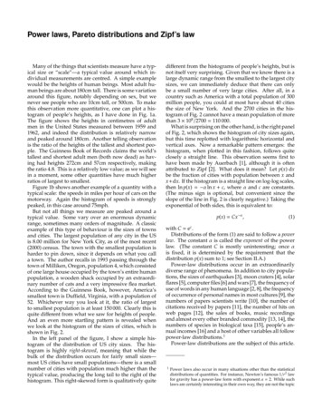
Power laws, Pareto distributions and Zipf’s law8In the author’s opinion, the identification of someof the distributions in Fig. 4 as following power lawsshould be considered unconfirmed. While the powerlaw seems to be an excellent model for most of the datasets depicted, a tenable case could be made that the distributions of web hits and family names might have twodifferent power-law regimes with slightly different exponents.7 And the data for the numbers of copies ofbooks sold cover rather a small range—little more thanone decade horizontally. Nonetheless, one can, withoutstretching the interpretation of the data unreasonably,claim that power-law distributions have been observedin language, demography, commerce, information andcomputer sciences, geology, physics and astronomy, andthis on its own is an extraordinary 0100200300number of addressesabundance(c)410210B. Distributions that do not follow a power lawPower-law distributions are, as we have seen, impressively ubiquitous, but they are not the only form ofbroad distribution. Lest I give the impression that everything interesting follows a power law, let me emphasizethat there are quite a number of quantities with highlyright-skewed distributions that nonetheless do not obeypower laws. A few of them, shown in Fig. 5, are thefollowing:(a) The abundance of North American bird species,which spans over five orders of magnitude butis probably distributed according to a log-normal.A log-normally distributed quantity is one whoselogarithm is normally distributed; see Sec
power-law distributions.1 Power-law distributions are the subject of this article. 1 Power laws also occur in many situations other than the statistical distributions of quantities. For instance, Newton’s famous 1 r2 law for gravity has a power-law form with exponent 2. While such laws are certainly interesting in their own way, they are not .File Size: 1MBPage Count: 27