WIXLIB

CONTENTS7.6 Linear Regression7.6.1 Prediction7.6.2 Goodness of Fit7.6.3 The Sample Correlation Coefficient7.6.4 Spearman’s Correlation Coefficient7.7 The General Linear Modelxiii4264344354374414438 Stochastic Processes8.1 Introduction8.2 Discrete -Time Markov Chains8.2.1 Time Dynamics of a Markov Chain8.2.2 Classification of States8.2.3 Stationary Distributions8.2.4 Convergence to the Stationary Distribution8.3 Random Walks and Branching Processes8.3.1 The Simple Random Walk8.3.2 Multidimensional Random Walks8.3.3 Branching Processes8.4 Continuous -Time Markov Chains8.4.1 Stationary Distributions and Limit Distributions8.4.2 Birth–Death Processes8.4.3 Queueing Theory8.4.4 Further Properties of Queueing Systems8.5 Martingales8.5.1 Martingale Convergence8.5.2 Stopping Times8.6 Renewal Processes8.6.1 Asymptotic Properties8.7 Brownian Motion8.7.1 Hitting Times8.7.2 Variations of the Brownian 1504506508510515517522525528Appendix A Tables541Appendix B Answers to Selected Problems551References563

xivIndexCONTENTS565

1Basic Probability Theory1.1 INTRODUCTIONProbability theory is the mathematics of randomness. This statement immediatelyinvites the question “What is randomness?” This is a deep question that we cannotattempt to answer without invoking the disciplines of philosophy, psychology, mathematical complexity theory, and quantum physics, and still there would most likelybe no completely satisfactory answer. For our purposes, an informal definition ofrandomness as “what happens in a situation where we cannot predict the outcomewith certainty” is sufficient. In many cases, this might simply mean lack of information. For example, if we flip a coin, we might think of the outcome as random.It will be either heads or tails, but we cannot say which, and if the coin is fair, webelieve that both outcomes are equally likely. However, if we knew the force fromthe fingers at the flip, weight and shape of the coin, material and shape of the tablesurface, and several other parameters, we would be able to predict the outcome withcertainty, according to the laws of physics. In this case we use randomness as a wayto describe uncertainty due to lack of information. 1Next question: “What is probability?” There are two main interpretations ofprobability, one that could be termed “objective” and the other “subjective.” The firstis the interpretation of a probability as a limit of relative frequencies; the second, asa degree of belief. Let us briefly describe each of these.1 Toquote the French mathematician Pierre-Simon Laplace, one of the first to develop a mathematicaltheory of probability: “Probability is composed partly of our ignorance, partly of our knowledge.”1

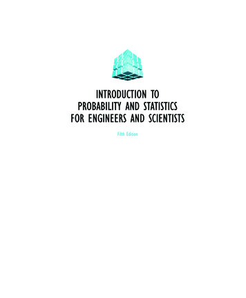
2BASIC PROBABILITY THEORYFor the first interpretation, suppose that we have an experiment where we areinterested in a particular outcome. We can repeat the experiment over and over andeach time record whether we got the outcome of interest. As we proceed, we countthe number of times that we got our outcome and divide this number by the number oftimes that we performed the experiment. The resulting ratio is the relative frequencyof our outcome. As it can be observed empirically that such relative frequencies tendto stabilize as the number of repetitions of the experiment grows, we might think ofthe limit of the relative frequencies as the probability of the outcome. In mathematicalnotation, if we consider n repetitions of the experiment and if Sn of these gave ouroutcome, then the relative frequency would be fn Sn /n, and we might say thatthe probability equals limn fn . Figure 1.1 shows a plot of the relative frequencyof heads in a computer simulation of 100 hundred coin flips. Notice how there issignificant variation in the beginning but how the relative frequency settles in toward12 quickly.The second interpretation, probability as a degree of belief, is not as easily quantified but has obvious intuitive appeal. In many cases, it overlaps with the previousinterpretation, for example, the coin flip. If we are asked to quantify our degree ofbelief that a coin flip gives heads, where 0 means “impossible” and 1 means “withcertainty,” we would probably settle for 12 unless we have some specific reason tobelieve that the coin is not fair. In some cases it is not possible to repeat the experiment in practice, but we can still imagine a sequence of repetitions. For example, ina weather forecast you will often hear statements like “there is a 30% chance of raintomorrow.” Of course, we cannot repeat the experiment; either it rains tomorrow or itdoes not. The 30% is the meteorologist’s measure of the chance of rain. There is stilla connection to the relative frequency approach; we can imagine a sequence of dayswith similar weather conditions, same time of year, and so on, and that in roughly30% of the cases, it rains the following day.The “degree of belief” approach becomes less clear for statements such as “theRiemann hypothesis is true” or “there is life on other planets.” Obviously theseare statements that are either true or false, but we do not know which, and it is not11/20020406080100Fig. 1.1 Consecutive relative frequencies of heads in 100 coin flips.

SAMPLE SPACES AND EVENTS3unreasonable to use probabilities to express how strongly we believe in their truth. It isalso obvious that different individuals may assign completely different probabilities.How, then, do we actually define a probability? Instead of trying to use any ofthese interpretations, we will state a strict mathematical definition of probability. Theinterpretations are still valid to develop intuition for the situation at hand, but insteadof, for example, assuming that relative frequencies stabilize, we will be able to provethat they do, within our theory.1.2 SAMPLE SPACES AND EVENTSAs mentioned in the introduction, probability theory is a mathematical theory todescribe and analyze situations where randomness or uncertainty are present. Anyspecific such situation will be referred to as a random experiment. We use the term“experiment” in a wide sense here; it could mean an actual physical experiment suchas flipping a coin or rolling a die, but it could also be a situation where we simplyobserve something, such as the price of a stock at a given time, the amount of rain inHouston in September, or the number of spam emails we receive in a day. After theexperiment is over, we call the result an outcome. For any given experiment, there isa set of possible outcomes, and we state the following definition.Definition 1.2.1. The set of all possible outcomes in a random experiment iscalled the sample space, denoted S.Here are some examples of random experiments and their associated sample spaces.Example 1.2.1. Roll a die and observe the number.Here we can get the numbers 1 through 6, and hence the sample space isS {1, 2, 3, 4, 5, 6}Example 1.2.2. Roll a die repeatedly and count the number of rolls it takes until thefirst 6 appears.Since the first 6 may come in the first roll, 1 is a possible outcome. Also, we may failto get 6 in the first roll and then get 6 in the second, so 2 is also a possible outcome. Ifwe continue this argument we realize that any positive integer is a possible outcomeand the sample space isS {1, 2, .}

4BASIC PROBABILITY THEORYthe set of positive integers.Example 1.2.3. Turn on a lightbulb and measure its lifetime, that is, the time untilit fails.Here it is not immediately clear what the sample space should be, since it depends onhow accurately we can measure time. The most convenient approach is to note thatthe lifetime, at least in theory, can assume any nonnegative real number and chooseas the sample spaceS [0, )where the outcome 0 means that the lightbulb is broken to start with.In these three examples, we have sample spaces of three different kinds. The firstis finite, meaning that it has a finite number of outcomes, whereas the second andthird are infinite. Although they are both infinite, they are different in the sense thatone has its points separated, {1, 2, .} and the other is an entire continuum of points.We call the first type countable infinity and the second uncountable infinity. We willreturn to these concepts later as they turn out to form an important distinction.In the examples above, the outcomes are always numbers and hence the samplespaces are subsets of the real line. Here are some examples of other types of samplespaces.Example 1.2.4. Flip a coin twice and observe the sequence of heads and tails.With H denoting heads and T denoting tails, one possible outcome is HT , whichmeans that we get heads in the first flip and tails in the second. Arguing like this,there are four possible outcomes and the sample space isS {HH, HT, TH, T T }Example 1.2.5. Throw a dart at random on a dart board of radius r.If we think of the board as a disk in the plane with center at the origin, an outcome isan ordered pair of real numbers (x, y), and we can describe the sample space asS {(x, y) : x2 y 2 r2 }

SAMPLE SPACES AND EVENTS5Once we have described an experiment and its sample space, we want to be able tocompute probabilities of the various things that may happen. What is the probabilitythat we get 6 when we roll a die? That the first 6 does not come before the fifth roll?That the lightbulb works for at least 1500 hours? That our dart hits the bull’s eye?Certainly we need to make further assumptions to be able to answer these questions,but before that, we realize that all these questions have something in common. Theyall ask for probabilities of either single outcomes or groups of outcomes. Mathematically, we can describe these as subsets of the sample space.Definition 1.2.2. A subset of S, A S, is called an event.Note the choice of words here. The terms “outcome” and “event” reflect the factthat we are describing things that may happen in real life. Mathematically, theseare described as elements and subsets of the sample space. This duality is typicalfor probability theory; there is a verbal description and a mathematical descriptionof the same situation. The verbal description is natural when real-world phenomenaare described and the mathematical formulation is necessary to develop a consistenttheory. See Table 1.1 for a list of set operations and their verbal description.Example 1.2.6. If we roll a die and observe the number, two possible events are thatwe get an odd outcome and that we get at least 4. If we view these as subsets of thesample space we getA {1, 3, 5} and B {4, 5, 6}If we want to use the verbal description we might write this asA {odd outcome} and B {at least 4}We always use “or” in its nonexclusive meaning; thus, “A or B occurs” includes thepossibility that both occur. Note that there are different ways to express combinationsof events; for example, A \ B A B c and (A B)c Ac B c . The latter isknown as one of De Morgan’s laws, and we state these without proof together withsome other basic set theoretic rules.

6BASIC PROBABILITY THEORYTable 1.1 Basic set operations and their verbal description.Notation Mathematical descriptionA BVerbal descriptionThe union of A and BA or B (or both) occursA BAcThe intersection of A and BThe complement of ABoth A and B occurA does not occurA\BØThe difference between A and BThe empty setA occurs but not BImpossible eventProposition 1.2.1. Let A, B, and C be events. Then(a) (Distributive Laws)(A B) C (A C) (B C)(A B) C (A C) (B C)(b) (De Morgan’s Laws) (A B)c Ac B c(A B)c Ac B cAs usual when dealing with set theory, Venn diagrams are useful. See Figure 1.2 foran illustration of some of the set operations introduced above. We will later return tohow Venn diagrams can be used to calculate probabilities. If A and B are such thatA B Ø, they are said to be disjoint or mutually exclusive. In words, this meansthat they cannot both occur simultaneously in the experiment.As we will often deal with unions of more than two or three events, we need moregeneral versions of the results given above. Let us first introduce some notation. IfA1 , A2 , ., An is a sequence of events, we denoten[Ak A1 A2 · · · Ann\Ak A1 A2 · · · Ank 1the union of all the Ak andk 1the intersection of all the Ak . In words, these are the events that at least one of theAk occurs and that all the Ak occur, respectively. The distributive and De Morgan’s

THE AXIOMS OF PROBABILITYABA7BB\AA BFig. 1.2 Venn diagrams of the intersection and the difference between events.laws extend in the obvious way, for example!cnn\[AckAk k 1k 1It is also natural to consider infinite unions and intersections. For example, in Example1.2.2, the event that the first 6 comes in an odd roll is the infinite union {1} {3} {5} · · · and we can use the same type of notation as for finite unions and write{first 6 in odd roll} [{2k 1}k 1For infinite unions and intersections, distributive and De Morgan’s laws still extendin the obvious way.1.3 THE AXIOMS OF PROBABILITYIn the previous section, we laid the basis for a theory of probability by describing random experiments in terms of the sample space, outcomes, and events. As mentioned,we want to be able to compute probabilities of events. In the introduction, we mentioned two different interpretations of probability: as a limit of relative frequenciesand as a degree of belief. Since our aim is to build a consistent mathematical theory,as widely applicable as possible, our definition of probability should not depend onany particular interpretation. For example, it makes intuitive sense to require a probability to always be less than or equal to one (or equivalently, less than or equal to100%). You cannot flip a coin 10 times and get 12 heads. Also, a statement such as “Iam 150% sure that it will rain tomorrow” may be used to express extreme pessimismregarding an upcoming picnic but is certainly not sensible from a logical point ofview. Also, a probability should be equal to one (or 100%), when there is absolutecertainty, regardless of any particular interpretation.Other properties must hold as well. For example, if you think there is a 20% chancethat Bob is in his house, a 30% chance that he is in his backyard, and a 50% chance

8BASIC PROBABILITY THEORYthat he is at work, then the chance that he is at home is 50%, the sum of 20% and30%. Relative frequencies are also additive in this sense, and it is natural to demandthat the same rule apply for probabilities.We now give a mathematical definition of probability, where it is defined as a realvalued function of the events, satisfying three properties, which we refer to as theaxioms of probability. In the light of the discussion above, they should be intuitivelyreasonable.Definition 1.3.1. (Axioms of Probability). A probability measure is afunction P , which assigns to each event A a number P (A) satisfying(a) 0 P (A) 1(b) P (S) 1(c) If A1 , A2 , . is a sequence of pairwise disjoint events, that is, if i 6 j,then Ai Aj Ø, then! X[PP (Ak )Ak k 1k 1We read P (A) as “the probability of A.” Note that a probability in this sense is areal number between 0 and 1 but we will occasionally also use percentages so that,for example, the phrases “The probability is 0.2” and “There is a 20% chance” meanthe same thing.2The third axiom is the most powerful assumption when it comes to deducing properties and further results. Some texts prefer to state the third axiom for finite unionsonly, but since infinite unions naturally arise even in simple examples, we choosethis more general version of the axioms. As it turns out, the finite case follows asa consequence of the infinite. We next state this in a proposition and also that theempty set has probability zero. Although intuitively obvious, we must prove that itfollows from the axioms. We leave this as an exercise.2 Ifthe sample space is very large, it may be impossible to assign probabilities to all events. The class ofevents then needs to be restricted to what is called a σ-field. For a more advanced treatment of probabilitytheory, this is a necessary restriction, but we can safely disregard this problem.

THE AXIOMS OF PROBABILITY9Proposition 1.3.1. Let P be a probability measure. Then(a) P (Ø) 0(b) If A1 , ., An are pairwise disjoint events, thenP(n[Ak ) k 1nXP (Ak )k 1In particular, if A and B are disjoint, then P (A B) P (A) P (B). In general,unions need not be disjoint and we next show how to compute the probability ofa union in general, as well as prove some other basic properties of the probabilitymeasure.Proposition 1.3.2. Let P be a probability measure on some sample space Sand let A and B be events. Then(a) P (Ac ) 1 P (A)(b) P (A \ B) P (A) P (A B)(c) P (A B) P (A) P (B) P (A B)(d) If A B, then P (A) P (B)Proof. We prove (b) and (c), and leave (a) and (d) as exercises. For (b), note thatA (A B) (A \ B), which is a disjoint union, and Proposition 1.3.1 givesP (A) P (A B) P (A \ B)which proves the assertion. For (c), we write A B A (B \ A), which is adisjoint union, and we getP (A B) P (A) P (B \ A) P (A) P (B) P (A B)by part (b).Note how we repeatedly used Proposition 1.3.1(b), the finite version of the third axiom. In Proposition 1.3.2(c), for example, the events A and B are not necessarily

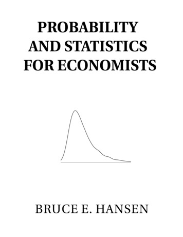
10BASIC PROBABILITY THEORYdisjoint but we can represent their union as a union of other events that are disjoint,thus allowing us to apply the third axiom.Example 1.3.1. Mrs Boudreaux and Mrs Thibodeaux are chatting over their fencewhen the new neighbor walks by. He is a man in his sixties with shabby clothes and adistinct smell of cheap whiskey. Mrs B, who has seen him before, tells Mrs T that heis a former Louisiana state senator. Mrs T finds this very hard to believe. “Yes,” saysMrs B, “he is a former state senator who got into a scandal long ago, had to resignand started drinking.” “Oh,” says Mrs T, “that sounds more probable.” “No,” saysMrs B, “I think you mean less probable.”Actually, Mrs B is rig

It is now more than a year later, and the book has been written. The first three chapters develop probability theory and introduce the axioms of probability, random variables, and joint distributions. The following two chapters are shorter and of an “introduction to” nature: