Transcription
NumPy User GuideRelease 1.18.4Written by the NumPy communityMay 24, 2020
CONTENTS1Setting up32Quickstart tutorial93NumPy basics334Miscellaneous975NumPy for Matlab users1036Building from source1117Using NumPy C-API115Python Module Index163Index165i
ii
NumPy User Guide, Release 1.18.4This guide is intended as an introductory overview of NumPy and explains how to install and make use of the mostimportant features of NumPy. For detailed reference documentation of the functions and classes contained in thepackage, see the reference.CONTENTS1
NumPy User Guide, Release 1.18.42CONTENTS
CHAPTERONESETTING UP1.1 What is NumPy?NumPy is the fundamental package for scientific computing in Python. It is a Python library that provides a multidimensional array object, various derived objects (such as masked arrays and matrices), and an assortment of routines forfast operations on arrays, including mathematical, logical, shape manipulation, sorting, selecting, I/O, discrete Fouriertransforms, basic linear algebra, basic statistical operations, random simulation and much more.At the core of the NumPy package, is the ndarray object. This encapsulates n-dimensional arrays of homogeneousdata types, with many operations being performed in compiled code for performance. There are several importantdifferences between NumPy arrays and the standard Python sequences: NumPy arrays have a fixed size at creation, unlike Python lists (which can grow dynamically). Changing thesize of an ndarray will create a new array and delete the original. The elements in a NumPy array are all required to be of the same data type, and thus will be the same size inmemory. The exception: one can have arrays of (Python, including NumPy) objects, thereby allowing for arraysof different sized elements. NumPy arrays facilitate advanced mathematical and other types of operations on large numbers of data. Typically, such operations are executed more efficiently and with less code than is possible using Python’s built-insequences. A growing plethora of scientific and mathematical Python-based packages are using NumPy arrays; thoughthese typically support Python-sequence input, they convert such input to NumPy arrays prior to processing,and they often output NumPy arrays. In other words, in order to efficiently use much (perhaps even most)of today’s scientific/mathematical Python-based software, just knowing how to use Python’s built-in sequencetypes is insufficient - one also needs to know how to use NumPy arrays.The points about sequence size and speed are particularly important in scientific computing. As a simple example,consider the case of multiplying each element in a 1-D sequence with the corresponding element in another sequenceof the same length. If the data are stored in two Python lists, a and b, we could iterate over each element:c []for i in range(len(a)):c.append(a[i]*b[i])This produces the correct answer, but if a and b each contain millions of numbers, we will pay the price for theinefficiencies of looping in Python. We could accomplish the same task much more quickly in C by writing (for claritywe neglect variable declarations and initializations, memory allocation, etc.)for (i 0; i rows; i ): {c[i] a[i]*b[i];}3
NumPy User Guide, Release 1.18.4This saves all the overhead involved in interpreting the Python code and manipulating Python objects, but at theexpense of the benefits gained from coding in Python. Furthermore, the coding work required increases with thedimensionality of our data. In the case of a 2-D array, for example, the C code (abridged as before) expands tofor (i 0; i rows; i ): {for (j 0; j columns; j ): {c[i][j] a[i][j]*b[i][j];}}NumPy gives us the best of both worlds: element-by-element operations are the “default mode” when an ndarray isinvolved, but the element-by-element operation is speedily executed by pre-compiled C code. In NumPyc a * bdoes what the earlier examples do, at near-C speeds, but with the code simplicity we expect from something based onPython. Indeed, the NumPy idiom is even simpler! This last example illustrates two of NumPy’s features which arethe basis of much of its power: vectorization and broadcasting.1.1.1 Why is NumPy Fast?Vectorization describes the absence of any explicit looping, indexing, etc., in the code - these things are taking place,of course, just “behind the scenes” in optimized, pre-compiled C code. Vectorized code has many advantages, amongwhich are: vectorized code is more concise and easier to read fewer lines of code generally means fewer bugs the code more closely resembles standard mathematical notation (making it easier, typically, to correctly codemathematical constructs) vectorization results in more “Pythonic” code. Without vectorization, our code would be littered with inefficientand difficult to read for loops.Broadcasting is the term used to describe the implicit element-by-element behavior of operations; generally speaking,in NumPy all operations, not just arithmetic operations, but logical, bit-wise, functional, etc., behave in this implicitelement-by-element fashion, i.e., they broadcast. Moreover, in the example above, a and b could be multidimensionalarrays of the same shape, or a scalar and an array, or even two arrays of with different shapes, provided that the smallerarray is “expandable” to the shape of the larger in such a way that the resulting broadcast is unambiguous. For detailed“rules” of broadcasting see numpy.doc.broadcasting.1.1.2 Who Else Uses NumPy?NumPy fully supports an object-oriented approach, starting, once again, with ndarray. For example, ndarray is aclass, possessing numerous methods and attributes. Many of its methods are mirrored by functions in the outermost NumPy namespace, allowing the programmer to code in whichever paradigm they prefer. This flexibility hasallowed the NumPy array dialect and NumPy ndarray class to become the de-facto language of multi-dimensionaldata interchange used in Python.4Chapter 1. Setting up
NumPy User Guide, Release 1.18.41.2 Installing NumPyIn most use cases the best way to install NumPy on your system is by using a pre-built package for your operatingsystem. Please see https://scipy.org/install.html for links to available options.For instructions on building for source package, see Building from source. This information is useful mainly foradvanced users.1.3 Troubleshooting ImportErrorNote: Since this information may be updated regularly, please ensure you are viewing the most up-to-date version.1.3.1 ImportErrorIn certain cases a failed installation or setup issue can cause you to see the following error message:IMPORTANT: PLEASE READ THIS FOR ADVICE ON HOW TO SOLVE THIS ISSUE!Importing the numpy c-extensions failed. This error can happen fordifferent reasons, often due to issues with your setup.The error also has additional information to help you troubleshoot: Your Python version Your NumPy versionPlease check both of these carefully to see if they are what you expect. You may need to check your PATH orPYTHONPATH environment variables (see Check Environment Variables below).The following sections list commonly reported issues depending on your setup. If you have an issue/solution that youthink should appear please open a NumPy issue so that it will be added.There are a few commonly reported issues depending on your system/setup. If none of the following tips help you,please be sure to note the following: how you installed Python how you installed NumPy your operating system whether or not you have multiple versions of Python installed if you built from source, your compiler versions and ideally a build logwhen investigating further and asking for support.1.2. Installing NumPy5
NumPy User Guide, Release 1.18.4Using Python from conda (Anaconda)Please make sure that you have activated your conda environment. See also the conda user-guide.Using Anaconda/conda Python within PyCharmThere are fairly common issues when using PyCharm together with Anaconda, please see the PyCharm supportRaspberry PiThere are sometimes issues reported on Raspberry Pi setups when installing using pip3 install (or pip install).These will typically mention:libf77blas.so.3: cannot open shared object file: No such file or directoryThe solution will be to either:sudo apt-get install libatlas-base-devto install the missing libraries expected by the self-compiled NumPy (ATLAS is a possible provider of linear algebra).Alternatively use the NumPy provided by Raspbian. In which case run:pip3 uninstall numpy # remove previously installed versionapt install python3-numpyDebug build on WindowsRather than building your project in DEBUG mode on windows, try building in RELEASE mode with debug symbolsand no optimization. Full DEBUG mode on windows changes the names of the DLLs python expects to find, so ifyou wish to truly work in DEBUG mode you will need to recompile the entire stack of python modules you work withincluding NumPyAll SetupsOccasionally there may be simple issues with old or bad installations of NumPy. In this case you may just try touninstall and reinstall NumPy. Make sure that NumPy is not found after uninstalling.Development SetupIf you are using a development setup, make sure to run git clean -xdf to delete all files not under version control(be careful not to lose any modifications you made, e.g. site.cfg). In many cases files from old builds may lead toincorrect builds.6Chapter 1. Setting up
NumPy User Guide, Release 1.18.4Check Environment VariablesIn general how to set and check your environment variables depends on your system. If you can open a correct pythonshell, you can also run the following in python:import osPYTHONPATH he PYTHONPATH is:", PYTHONPATH)PATH os.environ['PATH'].split(os.pathsep)print("The PATH is:", PATH)This may mainly help you if you are not running the python and/or NumPy version you are expecting to run.1.3. Troubleshooting ImportError7
NumPy User Guide, Release 1.18.48Chapter 1. Setting up
CHAPTERTWOQUICKSTART TUTORIAL2.1 PrerequisitesBefore reading this tutorial you should know a bit of Python. If you would like to refresh your memory, take a look atthe Python tutorial.If you wish to work the examples in this tutorial, you must also have some software installed on your computer. Pleasesee https://scipy.org/install.html for instructions.2.2 The BasicsNumPy’s main object is the homogeneous multidimensional array. It is a table of elements (usually numbers), all ofthe same type, indexed by a tuple of non-negative integers. In NumPy dimensions are called axes.For example, the coordinates of a point in 3D space [1, 2, 1] has one axis. That axis has 3 elements in it, so wesay it has a length of 3. In the example pictured below, the array has 2 axes. The first axis has a length of 2, the secondaxis has a length of 3.[[ 1., 0., 0.],[ 0., 1., 2.]]NumPy’s array class is called ndarray. It is also known by the alias array. Note that numpy.array is not thesame as the Standard Python Library class array.array, which only handles one-dimensional arrays and offersless functionality. The more important attributes of an ndarray object are:ndarray.ndim the number of axes (dimensions) of the array.ndarray.shape the dimensions of the array. This is a tuple of integers indicating the size of the array in each dimension. For a matrix with n rows and m columns, shape will be (n,m). The length of the shape tuple istherefore the number of axes, ndim.ndarray.size the total number of elements of the array. This is equal to the product of the elements of shape.ndarray.dtype an object describing the type of the elements in the array. One can create or specify dtype’s using standard Python types. Additionally NumPy provides types of its own. numpy.int32, numpy.int16, andnumpy.float64 are some examples.ndarray.itemsize the size in bytes of each element of the array. For example, an array of elements of type float64has itemsize 8 ( 64/8), while one of type complex32 has itemsize 4 ( 32/8). It is equivalent tondarray.dtype.itemsize.ndarray.data the buffer containing the actual elements of the array. Normally, we won’t need to use this attributebecause we will access the elements in an array using indexing facilities.9
NumPy User Guide, Release 1.18.42.2.1 An example import numpy as np a np.arange(15).reshape(3, 5) aarray([[ 0, 1, 2, 3, 4],[ 5, 6, 7, 8, 9],[10, 11, 12, 13, 14]]) a.shape(3, 5) a.ndim2 a.dtype.name'int64' a.itemsize8 a.size15 type(a) type 'numpy.ndarray' b np.array([6, 7, 8]) barray([6, 7, 8]) type(b) type 'numpy.ndarray' 2.2.2 Array CreationThere are several ways to create arrays.For example, you can create an array from a regular Python list or tuple using the array function. The type of theresulting array is deduced from the type of the elements in the sequences. import numpy as np a np.array([2,3,4]) aarray([2, 3, 4]) a.dtypedtype('int64') b np.array([1.2, 3.5, 5.1]) b.dtypedtype('float64')A frequent error consists in calling array with multiple numeric arguments, rather than providing a single list ofnumbers as an argument. a np.array(1,2,3,4) a np.array([1,2,3,4])# WRONG# RIGHTarray transforms sequences of sequences into two-dimensional arrays, sequences of sequences of sequences intothree-dimensional arrays, and so on. b np.array([(1.5,2,3), (4,5,6)]) barray([[ 1.5, 2. , 3. ],[ 4. , 5. , 6. ]])10Chapter 2. Quickstart tutorial
NumPy User Guide, Release 1.18.4The type of the array can also be explicitly specified at creation time: c np.array( [ [1,2], [3,4] ], dtype complex ) carray([[ 1. 0.j, 2. 0.j],[ 3. 0.j, 4. 0.j]])Often, the elements of an array are originally unknown, but its size is known. Hence, NumPy offers several functions tocreate arrays with initial placeholder content. These minimize the necessity of growing arrays, an expensive operation.The function zeros creates an array full of zeros, the function ones creates an array full of ones, and the functionempty creates an array whose initial content is random and depends on the state of the memory. By default, the dtypeof the created array is float64. np.zeros( (3,4) )array([[ 0., 0., 0., 0.],[ 0., 0., 0., 0.],[ 0., 0., 0., 0.]]) np.ones( (2,3,4), dtype np.int16 )array([[[ 1, 1, 1, 1],[ 1, 1, 1, 1],[ 1, 1, 1, 1]],[[ 1, 1, 1, 1],[ 1, 1, 1, 1],[ 1, 1, 1, 1]]], dtype int16) np.empty( (2,3) )array([[ 3.73603959e-262,6.02658058e-154,[ 5.30498948e-313,3.14673309e-307,# dtype can also be specified# uninitialized, output may vary6.55490914e-260],1.00000000e 000]])To create sequences of numbers, NumPy provides a function analogous to range that returns arrays instead of lists. np.arange( 10, 30, 5 )array([10, 15, 20, 25]) np.arange( 0, 2, 0.3 )array([ 0. , 0.3, 0.6, 0.9,1.2,1.5,# it accepts float arguments1.8])When arange is used with floating point arguments, it is generally not possible to predict the number of elementsobtained, due to the finite floating point precision. For this reason, it is usually better to use the function linspacethat receives as an argument the number of elements that we want, instead of the step: from numpy import pi np.linspace( 0, 2, 9 )array([ 0. , 0.25, 0.5 , 0.75, 1. x np.linspace( 0, 2*pi, 100 ) points f np.sin(x),# 9 numbers from 0 to 21.25, 1.5 , 1.75, 2. ])# useful to evaluate function at lots ofSee also:array, zeros, zeros like, ones, ones like, empty, empty like, arange, linspace, numpy.random.RandomState.rand, numpy.random.RandomState.randn, fromfunction, fromfile2.2. The Basics11
NumPy User Guide, Release 1.18.42.2.3 Printing ArraysWhen you print an array, NumPy displays it in a similar way to nested lists, but with the following layout: the last axis is printed from left to right, the second-to-last is printed from top to bottom, the rest are also printed from top to bottom, with each slice separated from the next by an empty line.One-dimensional arrays are then printed as rows, bidimensionals as matrices and tridimensionals as lists of matrices. a np.arange(6) print(a)[0 1 2 3 4 5] b np.arange(12).reshape(4,3) print(b)[[ 0 1 2][ 3 4 5][ 6 7 8][ 9 10 11]] c np.arange(24).reshape(2,3,4) print(c)[[[ 0 1 2 3][ 4 5 6 7][ 8 9 10 11]][[12 13 14 15][16 17 18 19][20 21 22 23]]]# 1d array# 2d array# 3d arraySee below to get more details on reshape.If an array is too large to be printed, NumPy automatically skips the central part of the array and only prints thecorners: print(np.arange(10000))[012 ., 9997 9998 9999] print(np.arange(10000).reshape(100,100))[[012 .,979899][ 100 101 102 ., 197 198 199][ 200 201 202 ., 297 298 299].,[9700 9701 9702 ., 9797 9798 9799][9800 9801 9802 ., 9897 9898 9899][9900 9901 9902 ., 9997 9998 9999]]To disable this behaviour and force NumPy to print the entire array, you can change the printing options usingset printoptions. np.set printoptions(threshold sys.maxsize)12# sys module should be importedChapter 2. Quickstart tutorial
NumPy User Guide, Release 1.18.42.2.4 Basic OperationsArithmetic operators on arrays apply elementwise. A new array is created and filled with the result. a np.array( [20,30,40,50] ) b np.arange( 4 ) barray([0, 1, 2, 3]) c a-b carray([20, 29, 38, 47]) b**2array([0, 1, 4, 9]) 10*np.sin(a)array([ 9.12945251, -9.88031624, 7.4511316 , -2.62374854]) a 35array([ True, True, False, False])Unlike in many matrix languages, the product operator * operates elementwise in NumPy arrays. The matrix productcan be performed using the @ operator (in python 3.5) or the dot function or method: A np.array( [[1,1],.[0,1]] ) B np.array( [[2,0],.[3,4]] ) A * Barray([[2, 0],[0, 4]]) A @ Barray([[5, 4],[3, 4]]) A.dot(B)array([[5, 4],[3, 4]])# elementwise product# matrix product# another matrix productSome operations, such as and * , act in place to modify an existing array rather than create a new one. a np.ones((2,3), dtype int) b np.random.random((2,3)) a * 3 aarray([[3, 3, 3],[3, 3, 3]]) b a barray([[ 3.417022 , 3.72032449, 3.00011437],[ 3.30233257, 3.14675589, 3.09233859]]) a b# b is not automatically converted to integer typeTraceback (most recent call last):.TypeError: Cannot cast ufunc add output from dtype('float64') to dtype('int64') with casting rule 'same kind'When operating with arrays of different types, the type of the resulting array corresponds to the more general or preciseone (a behavior known as upcasting). a np.ones(3, dtype np.int32) b np.linspace(0,pi,3)(continues on next page)2.2. The Basics13
NumPy User Guide, Release 1.18.4(continued from previous page) b.dtype.name'float64' c a b carray([ 1., 2.57079633, 4.14159265]) c.dtype.name'float64' d np.exp(c*1j) darray([ 0.54030231 0.84147098j, -0.84147098 0.54030231j,-0.54030231-0.84147098j]) d.dtype.name'complex128'Many unary operations, such as computing the sum of all the elements in the array, are implemented as methods ofthe ndarray class. a np.random.random((2,3)) aarray([[ 0.18626021, 0.34556073,[ 0.53881673, 0.41919451, a.sum()2.5718191614547998 a.min()0.1862602113776709 a.max()0.68521950039675950.39676747],0.6852195 ]])By default, these operations apply to the array as though it were a list of numbers, regardless of its shape. However,by specifying the axis parameter you can apply an operation along the specified axis of an array: b np.arange(12).reshape(3,4) barray([[ 0, 1, 2, 3],[ 4, 5, 6, 7],[ 8, 9, 10, 11]]) b.sum(axis 0)array([12, 15, 18, 21]) b.min(axis 1)array([0, 4, 8]) b.cumsum(axis 1)array([[ 0, 1, 3, 6],[ 4, 9, 15, 22],[ 8, 17, 27, 38]])14# sum of each column# min of each row# cumulative sum along each rowChapter 2. Quickstart tutorial
NumPy User Guide, Release 1.18.42.2.5 Universal FunctionsNumPy provides familiar mathematical functions such as sin, cos, and exp. In NumPy, these are called “universalfunctions”(ufunc). Within NumPy, these functions operate elementwise on an array, producing an array as output. B np.arange(3) Barray([0, 1, 2]) np.exp(B)array([ 1., 2.71828183, np.sqrt(B)array([ 0., 1., C np.array([2., -1., 4.]) np.add(B, C)array([ 2., 0., 6.])7.3890561 ])1.41421356])See also:all, any, apply along axis, argmax, argmin, argsort, average, bincount, ceil, clip, conj,corrcoef, cov, cross, cumprod, cumsum, diff, dot, floor, inner, inv, lexsort, max, maximum,mean, median, min, minimum, nonzero, outer, prod, re, round, sort, std, sum, trace, transpose,var, vdot, vectorize, where2.2.6 Indexing, Slicing and IteratingOne-dimensional arrays can be indexed, sliced and iterated over, much like lists and other Python sequences. a np.arange(10)**3 aarray([ 0,1,8, 27, 64, 125, 216, 343, 512, 729]) a[2]8 a[2:5]array([ 8, 27, 64]) a[:6:2] -1000# equivalent to a[0:6:2] -1000; from start to position 6, exclusive, set every 2nd element to -1000 aarray([-1000,1, -1000,27, -1000,125,216,343,512,729]) a[ : :-1]# reversed aarray([ 729,512,343,216,125, -1000,27, -1000,1, -1000]) for i in Multidimensional arrays can have one index per axis. These indices are given in a tuple separated by commas:2.2. The Basics15
NumPy User Guide, Release 1.18.4 def f(x,y):.return 10*x y. b np.fromfunction(f,(5,4),dtype int) barray([[ 0, 1, 2, 3],[10, 11, 12, 13],[20, 21, 22, 23],[30, 31, 32, 33],[40, 41, 42, 43]]) b[2,3]23 b[0:5, 1]# each row in the second column of barray([ 1, 11, 21, 31, 41]) b[ : ,1]# equivalent to the previous examplearray([ 1, 11, 21, 31, 41]) b[1:3, : ]# each column in the second and third row of barray([[10, 11, 12, 13],[20, 21, 22, 23]])When fewer indices are provided than the number of axes, the missing indices are considered complete slices: b[-1]array([40, 41, 42, 43])# the last row. Equivalent to b[-1,:]The expression within brackets in b[i] is treated as an i followed by as many instances of : as needed to representthe remaining axes. NumPy also allows you to write this using dots as b[i,.].The dots (.) represent as many colons as needed to produce a complete indexing tuple. For example, if x is anarray with 5 axes, then x[1,2,.] is equivalent to x[1,2,:,:,:], x[.,3] to x[:,:,:,:,3] and x[4,.,5,:] to x[4,:,:,5,:]. c np.array( [[[ 0, 1, 2],.[ 10, 12, 13]],.[[100,101,102],.[110,112,113]]]) c.shape(2, 2, 3) c[1,.]array([[100, 101, 102],[110, 112, 113]]) c[.,2]array([[ 2, 13],[102, 113]])# a 3D array (two stacked 2D arrays)# same as c[1,:,:] or c[1]# same as c[:,:,2]Iterating over multidimensional arrays is done with respect to the first axis: for row in b:.print(row).[0 1 2 3][10 11 12 13][20 21 22 23](continues on next page)16Chapter 2. Quickstart tutorial
NumPy User Guide, Release 1.18.4(continued from previous page)[30 31 32 33][40 41 42 43]However, if one wants to perform an operation on each element in the array, one can use the flat attribute which isan iterator over all the elements of the array: for element in 340414243See also:Indexing, arrays.indexing (reference), newaxis, ndenumerate, indices2.3 Shape Manipulation2.3.1 Changing the shape of an arrayAn array has a shape given by the number of elements along each axis: a np.floor(10*np.random.random((3,4))) aarray([[ 2., 8., 0., 6.],[ 4., 5., 1., 1.],[ 8., 9., 3., 6.]]) a.shape(3, 4)The shape of an array can be changed with various commands. Note that the following three commands all return amodified array, but do not change the original array: a.ravel() # returns the array, flattenedarray([ 2., 8., 0., 6., 4., 5., 1., 1., 8., 9., 3., a.reshape(6,2) # returns the array with a modified shape6.])(continues on next page)2.3. Shape Manipulation17
NumPy User Guide, Release 1.18.4(continued from previous page)array([[ 2., 8.],[ 0., 6.],[ 4., 5.],[ 1., 1.],[ 8., 9.],[ 3., 6.]]) a.T # returns the array, transposedarray([[ 2., 4., 8.],[ 8., 5., 9.],[ 0., 1., 3.],[ 6., 1., 6.]]) a.T.shape(4, 3) a.shape(3, 4)The order of the elements in the array resulting from ravel() is normally “C-style”, that is, the rightmost index “changesthe fastest”, so the element after a[0,0] is a[0,1]. If the array is reshaped to some other shape, again the array is treatedas “C-style”. NumPy normally creates arrays stored in this order, so ravel() will usually not need to copy its argument,but if the array was made by taking slices of another array or created with unusual options, it may need to be copied.The functions ravel() and reshape() can also be instructed, using an optional argument, to use FORTRAN-style arrays,in which the leftmost index changes the fastest.The reshape function returns its argument with a modified shape, whereas the ndarray.resize method modifiesthe array itself: aarray([[ 2., 8., 0.,[ 4., 5., 1.,[ 8., 9., 3., a.resize((2,6)) aarray([[ 2., 8., 0.,[ 1., 1., 8.,6.],1.],6.]])6.,9.,4.,3.,5.],6.]])If a dimension is given as -1 in a reshaping operation, the other dimensions are automatically calculated: a.reshape(3,-1)array([[ 2., 8., 0.,[ 4., 5., 1.,[ 8., 9., 3.,6.],1.],6.]])See also:ndarray.shape, reshape, resize, ravel18Chapter 2. Quickstart tutorial
NumPy User Guide, Release 1.18.42.3.2 Stacking together different arraysSeveral arrays can be stacked together along different axes: a np.floor(10*np.random.random((2,2))) aarray([[ 8., 8.],[ 0., 0.]]) b np.floor(10*np.random.random((2,2))) barray([[ 1., 8.],[ 0., 4.]]) np.vstack((a,b))array([[ 8., 8.],[ 0., 0.],[ 1., 8.],[ 0., 4.]]) np.hstack((a,b))array([[ 8., 8., 1., 8.],[ 0., 0., 0., 4.]])The function column stack stacks 1D arrays as columns into a 2D array. It is equivalent to hstack only for 2Darrays: from numpy import newaxis np.column stack((a,b))# with 2D arraysarray([[ 8., 8., 1., 8.],[ 0., 0., 0., 4.]]) a np.array([4.,2.]) b np.array([3.,8.]) np.column stack((a,b))# returns a 2D arrayarray([[ 4., 3.],[ 2., 8.]]) np.hstack((a,b))# the result is differentarray([ 4., 2., 3., 8.]) a[:,newaxis]# this allows to have a 2D columns vectorarray([[ 4.],[ 2.]]) np.column stack((a[:,newaxis],b[:,newaxis]))array([[ 4., 3.],[ 2., 8.]]) np.hstack((a[:,newaxis],b[:,newaxis]))# the result is the samearray([[ 4., 3.],[ 2., 8.]])On the other hand, the function ma.row stack is equivalent to vstack for any input arrays. In general, for arrayswith more than two dimensions, hstack stacks along their second axes, vstack stacks along their first axes, andconcatenate allows for an optional arguments giving the number of the axis along which the concatenation shouldhappen.NoteIn complex cases, r and c are useful for creating arrays by stacking numbers along one axis. They allow the use ofrange literals (“:”) np.r [1:4,0,4]array([1, 2, 3, 0, 4])2.3. Shape Manipulation19
NumPy User Guide, Release 1.18.4When used with arrays as arguments, r and c are similar to vstack and hstack in their default behavior, butallow for an optional argument giving the number of the axis along which to concatenate.See also:hstack, vstack, column stack, concatenate, c , r2.3.3 Splitting one array into several smaller onesUsing hsplit, you can split an array along its horizontal axis, either by specifying the number of equally shapedarrays to return, or by specifying the columns after which the division should occur: a np.floor(10*np.random.random((2,12))) aarray([[ 9., 5., 6., 3., 6., 8., 0., 7., 9., 7., 2., 7.],[ 1., 4., 9., 2., 2., 1., 0., 6., 2., 2., 4., 0.]]) np.hsplit(a,3)# Split a into 3[array([[ 9., 5., 6., 3.],[ 1., 4., 9., 2.]]), array([[ 6., 8., 0., 7.],[ 2., 1., 0., 6.]]), array([[ 9., 7., 2., 7.],[ 2., 2., 4., 0.]])] np.hsplit(a,(3,4))# Split a after the third and the fourth column[array([[ 9., 5., 6.],[ 1., 4., 9.]]), array([[ 3.],[ 2.]]), array([[ 6., 8., 0., 7., 9., 7., 2., 7.],[ 2., 1., 0., 6., 2., 2., 4., 0.]])]vsplit splits along the vertical axis, and array split allows one to specify along which axis to split.2.4 Copies and ViewsWhen operating and manipulating arrays, their data is sometimes copied into a new array and sometimes not. This isoften a source of confusion for beginners. There are three cases:2.4.1 No Copy at AllSimple assignments make no copy of array objects or of their data. a np.arange(12) b a# no new object is created b is a# a and b are two names for the same ndarray objectTrue b.shape 3,4# changes the shape of a a.shape(3, 4)Python passes mutable objects as references, so function calls make no copy. def f(x):.print(id(x)). id(a)148293216# id is a unique identifier of an object(continues on next page)20Chapter 2. Quickstart tutorial
NumPy User Guide, Release 1.18.4(continued from previous page) f(a)1482932162.4.2 View or Shallow CopyDifferent array objects can share the same data. The view method creates a new array object that looks at the samedata. c a.view() c is aFalse c.base is aTrue c.flags.owndataFalse c.shape 2,6 a.shape(3, 4) c[0,4] 1234 aarray([[0,1,[1234,5,[8,9,# c is a view of the data owned by a# a's shape doesn't change# a's data changes2,6,10,3],7],11]])Slicing an array returns a view of it: s a[ : , 1:3] 1:3]" s[:] 10 s[:] 10 aarray([[0,10,[1234,10,[8,10,# spaces added for clarity; could also be written "s a[:,# s[:] is a view of s. Note the difference between s 10 and10,10,10,3],7],11]])2.4.3 Deep CopyThe copy method makes a complete copy of the array and its data. d a.copy() created d is aFalse d.base is aFalse d[0,0] 9999 aa
For detailed reference documentation of the functions and classes contained in the package, see the reference. CONTENTS 1. NumPy User Guide, Release 1.18.4 2 CONTENTS. CHAPTER ONE SETTING UP . same as the Standard Python Library class array.array, which only handles one-dimensional arrays and offers less functionality. The more important .
