Transcription
GENERAL ARTICLEBrownian Motion Problem: Random Walk andBeyondShama Sharma and VishwamittarA brief account of developments in the experimental and theoretical investigations of Brownian motion is presented. Interestingly, Einsteinwho did not like God’s game of playing dice forelectrons in an atom himself put forward a theoryof Brownian movement allowing God to play thedice. The vital role played by his random walkmodel in the evolution of non-equilibrium statistical mechanics and multitude of its applicationsis highlighted. Also included are the basics ofLangevin’s theory for Brownian motion.IntroductionBrownian motion is the temperature-dependent perpetual, irregular motion of the particles (of linear dimension of the order of 10¡6m) immersed in a fluid, causedby their continuous bombardment by the surroundingmolecules of much smaller size (Figure 1). This e ectwas first reported by the Dutch physician, chemist andengineer Jan Ingenhousz (1785), when he found thatfine powder of charcoal floating on alcohol surface exhibited a highly random motion. However, it got thename Brownian motion after Scottish botanist RobertBrown, who in 1828-29 published the results of his extensive studies on the incessant random movement oftiny particles like pollen grains, dust and soot suspendedin a fluid (Box 1). To begin with when experimentswere performed with pollen immersed in water, it wasthought that ubiquitous irregular motion was due to thelife of these grains. But this idea was soon discarded asthe observations remained unchanged even when pollenwas subjected to various killing treatments, liquids otherRESONANCE August 2005Shama Sharma iscurrently working aslecturer at DAV College,Punjab. She is working onsome problems innonequilibrium statisticalmechanics.Vishwamittar is professorin physics at PanjabUniversity, Chandigarhand his present researchactivities are innonequilibrium statisticalmechanics. He has writtenarticles on teaching ofphysics, history andphilosophy of physics.KeywordsBro w ni a n m otion, L a n g evin’sth e ory, r a ndom w a lk, stoch a stic processes, non- e q uilibriu mst a tistica l m ech a nics.49
GENERAL ARTICLEFigure 1. Brownian motionof a fine particle immersedin a fluid.than water were used and fine particles of glass, petrified wood, minerals, sand, etc were immersed in variousliquids. Furthermore, possible causes like vibrations ofbuilding or the laboratory table, convection currents inthe fluid, coagulation of particles, capillary forces, internal circulation due to uneven evaporation, currentsproduced by illuminating light, etc were considered butwere found to be untenable.An early realization of the consequences of the studies on Brownian motion was that it imposes limit onthe precision of measurements by small instruments asthese are under the influence of random impacts of thesurrounding air.Box 1. Observing the Brownian MotionOne can observe Brownian movement by looking through an optical microscope with magnification 103– 104 at a well illuminated sample of some colloidal solution (say milk drops put into water) or smokeparticles in air. Alternately, we can mount a small mirror (area 1 or 2 mm2) on a fine torsion fiber capableof rotation about a vertical axis (as in suspension type galvanometer) in a chamber having air pressure ofabout 10–2 torr and note the movement of the spot of light reflected from the mirror. The trace of the lightspot is manifestation of angular Brownian motion of the mirror.It may be pointed out that movement of dust particles in the air as seen in a beam of light through a windowis not an example of Brownian motion as these particles are too large and the random collisions with airmolecules are neither much imbalanced nor strong enough to cause Brownian movement.50RESONANCE August 2005
GENERAL ARTICLEIn 1863, Wiener attributed Brownian motion to molecular movement of the liquid and this viewpoint wassupported by Delsaux (1877-80) and Gouy (1888-95).On the basis of a series of experiments Gouy convincingly ruled out the exterior factors as causes of Brownian motion and argued in favour of contribution of thesurrounding fluid. He also discussed the connection between Brownian motion and Carnot’s principle and thereby brought out the statistical nature of the laws of thermodynamics. Such ideas put Brownian motion at theheart of the then prevalent controversial views aboutphilosophy of science. Then, in 1900 Bachelier obtaineda di usion equation for random processes and thus, atheory of Brownian motion in his PhD thesis on stockmarket fluctuation. Unfortunately, this work was notrecognized by the scientific community, including hissupervisor Poincaré, because it was in the field of economics and it did not involve any of the relevant physicalaspects.Eventually, Einstein in a number of research publications beginning in 1905 put forward an acceptable modelfor Brownian motion1 . His approach is known as ‘random walk’ or ‘drunkards walk’ formalism and uses thefluctuations in molecular collisions as the cause of Brownian movement. His work was followed by an almost similar expression for the time dependence of displacementof the Brownian particle by Smoluchowski in 1906, whostarted with a probability function for describing themotion of the particle. In 1908, Langevin gave a phenomenological theory of Brownian motion and obtainedessentially the same formulae for displacement of theparticle. Their results were experimentally verified byPerrin (1908 and onwards)2 using precise measurementson sedimentation in colloidal suspensions to determinethe Avogadro’s number. Later on, more accurate values of this constant and that of Boltzmann constant kwere found out by many workers by performing similarexperiments.RESONANCE August 2005In 1863, Wienerattributed Brownianmotion to molecularmovement of theliquid.1These are collected in the bookA l b ert Einst e in : Inv esti g a tionso n t h e t h e o ry o f Bro w n i a nMove m e nt edited with notes byR Furth (Dov e r Pu b lic a tio ns,Ne w York,1956).2Revie w article entitle d ‘Browni a n M ov e m e nt a n d M ol ecul a rRe a lity’ b a se d on his w ork h a sb e e n tr a nsl a t e d into En glish byF So d dy a n d p u b lish e d by T a ylor & Fr a ncis,London in 1910.51
GENERAL ARTICLEThe correctness ofthe random walkmodel andLangevin’s theorymade a very strongcase in favour ofmolecular kineticmodel of matter.The techniquesdeveloped for thetheory of Brownianmotion formcornerstones forinvestigating a varietyof phenomena.52The correctness of the random walk model and Langevin’s theory made a very strong case in favour of molecular kinetic model of matter and unleashed a wave ofactivity for a systematic development of dynamical theory of Brownian motion by Fokker, Planck, Uhlenbeck,Ornstein and several other scientists. As such, duringthe last 100 years, concerted e orts by a galaxy of physicists, mathematicians, chemists, etc have not only provided a proper mathematical foundation to the physicaltheory but have also led to extensive diverse applicationsof the techniques developed.The two basic ingredients of Einstein’s theory were: (i)the movement of the Brownian particle is a consequenceof continuous impacts of the randomly moving surrounding molecules of the fluid (the ‘noise’); (ii) these impactscan be described only probabilistically so that time evolution of the particle under observation is also probabilistic in nature. Phenomena of this type are referred toas stochastic processes in mathematics and these are essentially non-equilibrium or irreversible processes. Thus,Einstein’s theory laid the foundation of stochastic modeling of natural phenomena and formed the basis ofdevelopment of non-equilibrium statistical mechanics,wherein generally, the Brownian particle is replaced bya collective property of a macroscopic system. Consequently, the techniques developed for the theory ofBrownian motion form cornerstones for investigating avariety of phenomena (in di erent branches of scienceand engineering) that have their origin in the e ect ofnumerous unpredictable and may be unobservable eventswhose individual contribution to the observed feature isnegligible, but collective impact is observed in the formof rather rapidly varying stochastic forces and dampinge ect (see Box 2).The main mathematical aspect of the early theories ofBrownian motion was the ‘central limit theorem’, whicham- ounted to the assumption that for a su ciently largeRESONANCE August 2005
GENERAL ARTICLEBox 2. Brownian MotorsOne of the topics of current research activity employing these techniques is referred to as Brownian motors.This phrase is used for the systems rectifying the inescapable thermal noise to produce unidirectionalcurrent of particles in the presence of asymmetric potentials. Their study is relevant for understanding thephysical aspects involved in the movement of motor proteins, the design and construction of efficientmicroscopic motors, development of separation techniques for particles of micro- and nano-size, possibledirected transport of quantum entities like electrons or spin degrees of freedom in quantum dot arrays,molecular wires and nano-materials; and to the fundamental problems of thermodynamics and statisticalmechanics such as basing the second law of thermodynamics on statistical reasoning and depriving theMaxwell demon type devices of their mystique and the trade-off between entropy and information.number of steps, the distribution function for randomwalk is quite close to a Gaussian. However, since thetrajectory of a Brownian particle is random, it growsonly as square root of time3 and, therefore, one cannotdefine its derivative at a point. To handle this problem,N Wiener (1923) put forward a measure theory whichformed the basis of the so-called stable distributions orLevy distributions. As a follow-up of these and to givea firm footing to the theory of Brownian motion, Ito(1944), developed stochastic calculus and an alternativeto Brownian motion — the Geometrical Brownian motion. This, in turn, led to extensive modeling for thefinancial market, where the balance of supply and demand introduces a random character in the macroscopicprice evolution. Here the logarithm of the asset price isgoverned by the rules for Brownian motion. These aspects have enlarged the scope of applicability of theoretical methods far beyond Einstein’s random walks. Theseconcepts have been fruitfully exploited in a multitude ofphenomena in not only physics, chemistry and biologybut also physiology, economics, sociology and politics.The Random Walk Model for Brownian MotionWhile tottering along, a drunkard is not sure of his steps;these may be forward or backward or in any other direction. Besides, each step is independent of the onealreadyRESONANCE August 20053This result w ill b e o bt a in e d inth e n e xt s e ctio n of this a rticl e ;se e e q u a tion (8).The mainmathematical aspectof the early theoriesof Brownian motionwas the ‘central limittheorem’, whichstates that thedistribution functionfor random walk isquite close to aGaussian.53
GENERAL ARTICLEtaken. Thus, his motion is so irregular that nothingcan be predicted about the next step. All one can talkabout is the probability of his covering a specific distancein given time. Such a problem was originally solvedby Markov and therefore, such processes are known asMarkov processes. Einstein adopted this approach toobtain the probability of the Brownian particle coveringa particular distance in time t. The randomness of thedrunkard’s walk has given this treatment the name ‘random walk model’ and in the case of a Brownian particle,the steps of the walk are caused by molecular collisions.To simplify the derivation, we consider the problem inone-dimension along x-axis, taking the position of theparticle to be 0 at t 0 and x(t) at time t and makethe following assumptions.1. Each molecular impact on the particle under observation takes place after the same interval ¿0(10¡8 s) sothat the number of collisions in time t is n t/¿0 (ofthe order of 108).2. Each collision makes the Brownian particle jump bythe same distance which turns out, we will see, to beabout 1nm, for a particle of radius 1µm in a fluid withthe viscosity of water, at room temperature along eitherpositive or negative direction with equal probability and is much smaller than the displacement x(t) which weresolve through the microscope only on the scale of aµm of the particle.3. Successive jumps of the particle are independent ofeach other.4. At time t, the particle has net positive displacementx(t) (it could be equally well taken as negative) so thatout of n jumps, m( x(t)/ , of the order of 103) extrajumps have taken place in positive direction. Since nand m are quite large, these are taken as integers.54RESONANCE August 2005
GENERAL ARTICLEIn view of the four assumptions above, the total numberof positive and negative jumps, respectively, is (n m)/2and (n ¡ m)/2. Since the probability that n independent jumps, each with probability 1/2, have a particular sequence is (1/2)n , the probability of having m extrapositive jumps is given byP n(m) (1/2)(1/2)n{n!/[(n m)/2]![(n ¡ m)/2]!},(1)where the factor (1/2) comes from normalization § mPn (m) 1. While writing this expression, we have notused any restriction on n and m except that both areintegers. So it holds good even for small n and m. Notethat both n and m are either even or odd. As an illustration, if we consider 8 jumps, then the probabilitiesfor m 0, 2, 4 and 8 are 35/256, 7/64, 7/128 and 1/512,respectively.For large n we can use the approximation n! (2¼n)1/2(n/e)n, so that for large n and m, equation(1) finallybecomesPn (m) (1/2n)1/2 exp(¡m2/2n).(2)Substituting m x/ and n t/¿0, this yields theprobability for the particle to be found in the interval xto x dx at time t asP (x)dx (1/4¼Dt)1/2exp( ¡x2/4Dt)dx,(3)with D 2/2¿0 . It may be mentioned that taking m tobe large mathematically means that is infinitesimallysmall for a finite value of x. This aspect has enabledus to switch over from discrete step random walk to acontinuous variable x in the above expression.In order to understand the physical significance of thesymbol D, recall that if the linear number density ofsuspended particles in a fluid is N(x, t) and their concentration is di erent in di erent regions, di usion takesRESONANCE August 200555
GENERAL ARTICLEplace. This is governed by the di usion equationD0(@ 2 N(x, t)/@x2) @N(x, t)/@t,(4)where D0 is the di usion coe cient. Equation (4) hasone of the solutions aspN(x, t) (Ntot / {4¼D0 t})exp(¡x2 /4D0 t).(5)Here,Ntot Z1N(x, t)dx(6)¡1is the total number of particles along the x-axis. Obviously, N (x, t)/Ntot corresponds to P (x) if we identifyD as D0 , i.e, 2 /2¿0 as di usion coe cient. In otherwords, P (x) is a solution of the di usion equation meaning thereby that the random walk problem is intimatelyrelated with the phenomenon of di usion. In fact, therandom walk model is a microscopic phenomenon of diffusion.A look at (3) shows that the probability function describing the position of the particle at time t is Gaussianwith dispersion 2Dt (Figure 2) implying spread of thepeak width as square root of t. Furthermore, mean values of x(t) and x2(t) turn out to behx(t)i 0The proportionality ofroot mean squaredisplacement of theBrownian particle tothe square root oftime is a typicalconsequence of therandom nature of theprocess.56andhx2(t)i 2Dt.(7)Since hx(t)i 0, the physical quantity of interest ishx2 (t)i . So what one measures experimentally is theroot mean square displacement of the Brownian particlegiven byxrms hx2(t)i 1/2 (2Dt)1/2.(8)The proportionality of root mean square displacementof the Brownian particle to the square root of time is atypical consequence of the random nature of the processRESONANCE August 2005
GENERAL ARTICLE1.210.8Series1Series2Series30.60.40.2and is in contrast with the result of usual mechanicalpredictable and reversible motion where displacementvaries as t. For three dimensional motion, the aboveexpression becomeshr2(t)i hx2 (t)i hy2(t)i hz 2(t)i 6Dt.(9)From equation (7), we haveD h e 2. Plot of (4p Dt)1/2P(x) (equation(3)) versus xfor D 5.22 10–13 m2 s–1 andx varying from 5.0 mm to5.0 mm corresponding to tvalues 1s (the innermostcurve), 2s (the middlecurve), and 4s (the outermost curve ).(10)which connects the macroscopic quantity di usion constant D or D0 with the microscopic quantity the meansquare displacement due to jumps. It gives us a direct relationship between the di usion process, which isirreversible, and Brownian movement that has its origin in random collisions. In other words, irreversibilityhas something to do with the random fluctuating forcesacting on the Brownian particle due to impacts of themolecules of the surrounding fluid.RESONANCE August 200557
GENERAL ARTICLE4O n e such w e ll-inv e sti g a t e dto p ic is th a t of q u a ntu m r a nd o m w a lks – a n a tur a l e xt e nsion of cl assica l ra ndom w a lks.Thou g h th e m a in e m p h a sis inth e s e stu d i e s h a s b e e n o nbrin g in g out th e d iff e r e nc e s inth e ir b e h a viour a s com p a re dto th e cl a ssic a l a n a lo gs, it isb e li e v e d th a t this kn o w l e d g ewill b e h elpful in d evelopinga lgorithms th a t ca n b e run on aq u a n t u m co m p u t e r a s a n dw h e n it is pr a ctic a lly re a liz e d.The successful use of the concept of random walk in thetheory of Brownian motion encouraged physicists to exploit it in di erent fields involving stochastic processes.4Langevin’s Theory of Brownian MotionThe intimate relationship between irreversibility and randomness of collisions of the fluid molecules with theBrownian particle (mentioned above) prompted Langevin(1908) to put forward a more logical theory of Brownian movement. However, before proceeding further, wedigress to consider the motion of a hockey ball of massM being hit quickly by di erent players. Its motion isgoverned by two factors. The frictional force f d betweenthe surface of ball and the ground tends to slow it down,while the impact of the hit with the stick by a player increases its velocity. The e ect of the latter, of course, isquite random as its magnitude as well as direction depend upon the impulse of the hit. Since a hit lasts foronly a very short time, we represent the magnitude fj ofcorresponding force at time tj by a Dirac delta function( Box 3 ) of strength Cjfj (t) Cj (t ¡ tj ),(11)and write the equation of motion pertaining to this forceasM dv/dt fj .(12)To find the e ect of the hit in changing the velocity,we substitute (11) into (12), integrate on both the sideswith respect to time over a small time interval aroundtj and use the property of delta function to getM vj C j.(13)Here, vj is the change in velocity brought about bythe hit at time t tj. Now, the hits applied by di erentplayers can be in any direction, the total force exerted58RESONANCE August 2005
GENERAL ARTICLEBox 3. The Dirac Delta FunctionMany times we come across problems in which the sources or causes of the observed effects are nearlylocalized or almost instantaneous. Some such examples are : point charges and dipoles in electrostatics;impulsive forces in dynamics and acoustics; peaked voltages or currents in switching processes; nuclearinteractions, etc. To handle such situations, we use what is known as Dirac delta function. It represents aninfinitely sharply peaked function given, for one-dimensional case, by 0δ ( x x 0 ) x x0x x0but such that its integral over the whole range is normalized to unity : δ ( x x 0 )dx 1. Its most important property is that for a continuous function f(x) f (x )δ ( x x 0 ) dx f ( x0 ). Thus, δ (x – x0) acts as a sieve that selects from all possible values of f(x) its value at the point x0, wherethe δ function is peaked. Accordingly, the above result is sometimes called sifting property ofδ function.on the ball in a finite time interval will be obtained bysumming up the above expression over a sequence of hitsmade taking into account the directions of the hits. Thisforce can be written asfr (t) §j Cj Áj (t ¡ tj ),(14)where Á j is unit vector in the direction of hit at timet tj . The subscript r in (14) has been used to indicatethe randomness of the force vector. Thus, the total forceacting on the ball at any time t will be f d fr and itsequation of motion will readM dv/dt f d f r .(15)Furthermore, if a very large number of hits are appliedquickly over a long time interval as compared to theimpact time, all possible directions Áj will occur completely randomly with equal probability. Accordingly,RESONANCE August 200559
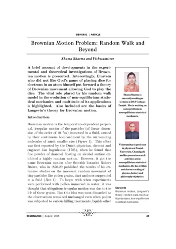
GENERAL ARTICLEFigure 3. A large Brownianparticle surrounded by randomly moving relativelysmaller molecules of thefluid.average value of fr will be zero, i.e.,hf r (t)i 0.Reverting to the Langevin’s theory, we consider Brownian particle in place of the hockey ball in the above illustration and make the following simplifying assumptions.1. The Brownian particle experiences a time-dependentforce f(t) only due to molecular impacts from the surrounding particles (Figure 3) and there is no other external force ( such as gravitational, Coulombic, etc.) actingon it.2. The force f(t) is made up of two parts: f d and f r (t).The former is an averaged out, systematic or steadyforce due to frictional or viscous drag of the fluid, whilethe latter is a highly fluctuating force or noise arisingfrom the irregular continuous bombardment by the fluidmolecules. The equation of motion of the particle isgiven by (15).3. The steady force fd is governed by the Stokes formula(Box 4) so thatfd ¡ v.60(16)RESONANCE August 2005
GENERAL ARTICLEBox 4. Stokes FormulaFollowing Stokes we assume that a perfectly rigid body (say, a sphere) with completely smooth surface andlinear dimension l is moving through an incompressible, viscous fluid ( viscosity η, density ρ ) having aninfinite extent in such a manner that there is no slip between the body and the layers of the fluid in itscontact, with such a speed v that the motion is streamlined and the Reynolds number R ( vlρ/η) is verysmall (strictly speaking vanishingly small), then the viscous drag force fd on the body is proportional tovelocity v, i.e. fd – γ v; and the constant γ depends on the geometry of the body. For example, it is 6πηafor a sphere of radius a and is 16 ηa for a plane circular disc of radius a moving perpendicular to its plane.Here, is viscous drag coe cient and1/ v / fd (17)is mobility of the Brownian particle. The drag coe cientdepends upon viscosity of the fluid, geometry as wellas size of the Brownian particle. For a spherical particleof radius a, 6¼ a.(18)4. The coe cient of viscous drag is a constant, havingthe same value in all parts of the fluid and at all times.5. The random force fr (t) is independent of v(t) andvaries extremely fast as compared to it so that over along time interval (much larger than the characteristicrelaxation time ¿), the average of f r (t) vanishes (as elaborated above for a hockey ball), i.e.,hfr (t)i 0.(19)This essentially amounts to saying that the collisionsare completely independent of each other or are uncorrelated.Substituting (16) into (15), we getM (dv/dt) ¡ v fr (t),RESONANCE August 2005(20)61
GENERAL ARTICLEwhere fr (t) satisfies the condition given in (19).This isthe celebrated Langevin equation for a free Brownianparticle. fr (t) is usually referred to as ‘stochastic force’;(20) is the stochastic equation of motion and is the basicequation used for describing a stochastic process. Thesolution to (20) readsZ t¡¡v(t) v(0)exp( t/¿ ) exp( t/¿ )exp(u/¿ )A(u)du,0(21)and gives us the drift velocity of the Brownian particle.Here,¿ M/ (22)is the relaxation time of the particle andA(t) fr (t)/M(23)is the stochastic force per unit mass of the Brownianparticle and is generally called ‘Langevin force’.It may be mentioned that the first term in (21) is thedamping term and it tries to exponentially reduce thevalue of v(t) to make it essentially dead. On the otherhand, the second term involving Langevin force or noisecreates a tendency for v(t) to spread out over a continually increasing range of values due to integration and,thus, keeping it alive. Consequently, the observed valueof drift velocity at any time t is an outcome of these twoopposing tendencies.From (19) and (23), it is clear that hA(t)i 0 so thatthe average value of drift velocity in (21) becomeshv(t)i v(0)exp(¡ t/¿ ).(24)Obviously, average drift velocity of the Brownian particle decays exponentially with a characteristic time ¿ tillit becomes zero. This is a typical result for dissipative62RESONANCE August 2005
GENERAL ARTICLEor irreversible processes. But, this is physically not acceptable as ultimately the particle must be in thermalequilibrium with its surroundings at ambient temperature and, therefore, cannot be at rest. So we considerh v2(t)i hv(t).v(t) i. Substituting for v(t) from (21)and using the fact that hA(t)i 0, we havehv2(t)i v2(0)exp(¡2t/¿) exp(¡2t/¿ ) Z tZ0t0exp(u1 u2)/¿ )K(u2 ¡ u1)du1du2,(25)whereK (u2 ¡ u1) hA(u1).A(u2)i.(26)It is called autocorrelation function for the Langevinforce A(u) and involves u2 ¡ u1 to emphasize the factthat for Brownian motion it depends upon the time interval u2 ¡ u1 rather than actual values of u1 and u2.We assume that K(u2 ¡ u1) is an even function of itsargument and is significant only for u2 almost equal tou1. Using these ideas when the double integral in (25)is evaluated, we get52222hv (t)i v (0) [v (1) ¡ v (0)][1 ¡ exp(¡2t/¼)].(27)5For d e t a ils of this ste p se eS t a tistic a l M ech a nics b y R KP a thri a list e d a t th e e n d .Here, hv2( 1)i is the mean square velocity of the Brownian particle for infinitely large value of t and is expectedto be the value corresponding to the situation when thesystem is in equilibrium at temperature T . Thus, fromequipartition theorem(1/2)M v2 (1) (3/2)kT.(28)As a special case if v2 (0) equals the equipartition value3kT /M, then hv2(t)i v2(0) 3kT /M implying thatif the system has attained statistical equilibrium then itwould continue to be so throughout.RESONANCE August 200563
GENERAL ARTICLEIt may be noted that multiplying (20) with r(t)/M,where r(t) is the instantaneous position of the Brownianparticle, we finally getd2hr 2i/dt2 (1/¿ )(dhr 2i/dt) 2h v2(t)i;(29)here h v2(t)i is given by (27). This second order di erential equation, on being solved, giveshr2 (t)i v2(0)¿ 2{1 ¡ exp(¡ t/¿ )}2 ¡ (3kT /M )¿ 2 {1 ¡ exp(¡t/¿)}{1 ¡ exp(¡ t/¿ )} (6kT ¿ /M)t. (30)For t very small as compared to ¿ it yieldshr2 (t) i v2(0)t2,(31)so that root mean square displacement rrms hr2(t)i1/2is proportional to t as for a reversible process. On theother hand, for t À ¿ , we gethr 2(t)i (6kT ¿ /m)t (6kT / )tThe Einstein relationgives a relationshipbetween the diffusioncoefficient andmobility of the particleand hence theviscosity of the fluid.(32)implying thatrrms (t) (6kT / )1/2t1/2 .(33)Expression (32) becomes identical to (9) if we takeD kT / ,(34)which in view of (18) readsThus, viscosity of amedium is aconsequence offluctuating forcesarising from theircontinuous andrandom motion and isan irreversiblephenomenon.64D kT /6¼ a(35)for a spherical Brownian particle. Equation (34) is usually known as ‘Einstein relation’. Obviously, it gives arelationship between the di usion coe cient and mobility of the particle and hence the viscosity of the fluid.Thus, viscosity of a medium is a consequence of fluctuating forces arising from their continuous and randommotion and is an irreversible phenomenon.RESONANCE August 2005
GENERAL ARTICLEAt this stage it is in order to mention one of the experimental observations by Perrin and Chaudesaigues.They studied the mean square displacement of gambogeparticles of radius 0.212 µm in a medium with viscosity 0.0012 Nm¡2 s and maintained at a temperature of186 K. The values found along the x-axis at times 30,60, 90 and 120 seconds, respectively, were 45, 86.5, 140,195 10¡12 m2 . These give the mean value of squareddisplacement for 30 seconds as 48.75 10¡12 m2. Now,from (7) and (35), we havehx2(t)i (kT t/3¼ a),(36)which on substituting the above listed values yields k 1.36 10¡23JK ¡1 . Clearly, it is quite close to the accepted value of the Boltzmann constant except that thedeviation is reasonably large.It may be mentioned that the Langevin equation (equation (20)) was based on the assumptions enumerated inthe beginning of this section. However, in a real systembeing used for the observation of Brownian motion, someexternal force fext (t) may be present; the viscous dragforce f d may be a function of higher powers of velocityor some other function of v(t); the drag coe cient maynot be a constant and rather may depend upon v, t oreven position. In such a case this equation is modifiedto a general formM (dv/dt) ¡ (v, x, t)F (v) f r (t) fext (t).(37)It is worthwhile to point out that the Langevin equations can also be obtained by assuming the Brownianparticle to be interacting bilinearly with a large number of harmonic oscillators constituting a heat bath6 .This approach yields explicit expressions for the dragforce f d as well as the stochastic force or noise fr (t) and,thus, provides better insight into their mechanism butstill does not make the theory very rigorous7 . The lattertask is achieved by using the so called master equationRESONANCE August 20056This d e riv a tion is g iv e n , e . g .,in a r
drunkard’s walk has given this treatment the name ‘ran-dom walk model’ and in the case of a Brownian particle, the steps of the walk are caused by molecular collisions. To simplify the derivation, we consider the problem in one-dimension along x-axis, taking the position of