Transcription
Glenforest Secondary SchoolExtended EssayProbability of a 45º Drunkard’s WalkDavid Kong2203-0033MathWord Count: 3814
ABSTRACTPAGE 2AbstractWe take a glimpse into higher level probability with the ‚random walk,‛ a particlemoving in random directions on a plane. The focus, however, is very specific: a veryparticular kind of random walk, as described by an ‚USA Mathematics TalentSearch‛ question,3/4/20. A particle is currently at the point (0, 3.5) on the plane and is movingtowards the origin. When the particle hits a lattice point (a point with integercoordinates), it turns with equal probability 45 to the left or to the right fromits current course. Find the probability that the particle reaches the x-axisbefore hitting the line y 6 USA (Mathematical Talent Search).We begin by considering a smaller model in order to develop theorems based aroundthe symmetrical nature of the particle’s movement. These theorems are applied tothe original question and by focusing on particular points of the particle’s motionand we solve a system of equations to reveal the answer to be. We then check thevalidity of our work by comparing the theoretical probability to the empiricalprobability as found by an excel program we later create.We then extend the problem to find that for a particle beginning downward at(0,4.5), the probability of reaching the x-axis before reaching y 8 is.Finally, we use the patterns from these smaller models to create a system ofequations which, when solved, gives the answers to much larger models, includingthe final assignment: finding the probability of reaching the x-axis before reachingy 50. Assuming the particle, again, begins halfway (0,25.5), this was found by ourexcel program to be around 0.555.269 wordsDavid Kong – 2203 033
ABSTRACTPAGE 3Table of ContentsAbstract . 21.0Introduction . 42.0Developing a Method . 73.0Creating an Excel Model . Error! Bookmark not defined.4.0Solving the Problem . 125.0Extending the Problem . 196.0Using Excel for Scalability . 297.0Conclusion . 438.0Works Cited . 469.0Acknowledgements . 4610.0Appendices . 47David Kong – 2203 033
1.01.0PAGE 4IntroductionIntroductionSimple probability almost always involves an event space and sample space. Eventhe more difficult questions, such as those involving binomial distribution can stillbe represented in the number of times of success over the number of successes andfailures.However, in higher level probability, questions are elevated to a point where thesample space is infinite. As a direct approach becomes impossible, these questionsare more difficult, and require original solutions. An integral part of higher levelprobability is the ‚random walk,‛ the study of a particle moving randomly in space.While applications of this field are numerous and significant, including the stockmarket and molecular movement (Brownian motion), it is outside the scope of thisessay. Instead we will thoroughly investigate one particular type of random walk todemonstrate the sort of treatment a question of this calibre requires.While our solution will include probability laws like that of ‚combined events,‛ ithas a surprisingly high reliance on other pre-calculus disciplines.From the USA Math Talent Search:3/4/20. A particle is currently at the point (0, 3.5) on the plane and is movingtowards the origin. When the particle hits a lattice point (a point with integercoordinates), it turns with equal probability 45 to the left or to the right fromits current course. Find the probability that the particle reaches the x-axisbefore hitting the line y 6 (Mathematical Talent Search).The following diagram elucidates the motion described above.David Kong – 2203 033
1.0PAGE 5IntroductionThe particle starts at (0,4),1 and begins its path down to (0,3). In this path, theparticle first turns right of its current path at a 45 angle, towards the lattice point(-1,2), where it turns right 45 again. The particle continues to make left and rightturns randomly until it hits y 6, where it terminates. This path is considered afailure.1.1 Definitions and Notation Let us define the event of the particle reaching y 0before y 6 a success, or winning. Let us refer to y 0 as the lower bound and y 6 asthe upper bound. Letrepresent the probability of winning given that theparticle is at point (x,y), and the upper bound is y a while the lower bound is y 0.As the question specifies ‘lattice points,’ a, x and y and all other variables orparameters introduced can be expected to be either integers or a subset of .Please note that our notation has a limitation in that it does not specify thedirection. For simplicity, directional information will not be denoted in ‘.’We only consider the most direct path a particle can take to (x,y). For example,can only represent the probability of a particle moving south because theparticle arrives in that situation in only one move whereas any other direction wouldrequire repositioning and thus many more moves. The reader will have access to1Although the question specifies that the particle starts at (0,3.5), we begin our paths on alattice point without altering the results in any way.David Kong – 2203 033
1.0PAGE 6Introductiongraphs which accompany the mathematical equations which explicitly show thedirection in question.The answer to our problem is expressed asthrough (0,3)., since the particle necessarily goesDavid Kong – 2203 033
2.0PAGE 7Developing a Method2.0Developing a MethodTo solve this problem, our strategy is to look at a smaller model.Particle bound by y 0 and y 4As the particle in the original problem began just above half, we will begin oursmaller model at (0,3). The first move will be down to (0,2) where it can either turnleft or right, and have these possible paths for the first five moves of the particle.Theorem 2.1where (d,e) and (f,g)are the twopossible progressions from (b,c).Proof. From a tree diagram,winning from (d,e)turning right to (d,e)losing from (d,e)at(b,c)wining from (f,g)turning left to (f,g)losing from (f,g)David Kong – 2203 033
2.0PAGE 8Developing a MethodThe probability of winning at (b,c) is therefore:Therefore the probability of winning on the first move,(2.1)However, notice from the diagram that the particle at (-1,1) is on a similar path asthe one at (1,1), just in the opposite direction.Theorem 2.2particle atVertical Line of Symmetry.given that thewhen flipped in the line x d shares the same path as.Proof. The particles atandhave congruent paths, which is easilyshown when one is flipped in the line x d. Therefore, their probabilities of successmust be equal.Sincewe can simplify Equation 2.1,David Kong – 2203 033
2.0PAGE 9Developing a MethodThis is useful because we can eliminate (-1,1) from our solution. In the diagrambelow, the orange path can be eliminated because for the same reason, we reason that.One method of findingsuch:would be to apply theorem 2.1 over and over again as(Theorem 2.2)()()(2.2)However, such a solution is unappealing and hard to follow. Instead, we will use astep counting method. Here is a graph for the interval. The endpoints, orthe points in Equation 2.2, are marked.David Kong – 2203 033
2.0PAGE 10Developing a MethodIdentifying the endpoints is important because each end point corresponds to a path,whose collective probabilities make up. In order for the particle to arrive atthe point, must turn in the correct direction at every junction. For example, aparticle at (4,4) arrives after turning left at each of the 3 junctions.2 The probabilityof passing the junction on the correct trajectory is 0.5 so( )Sinceis the combination of the probabilities at all possible endpoints,( )( )2( )Please note that (0,2) and (3,3) are not counted as junctions. As Thorem 2.2 points out, nomatter if the particle moves left or right at these point, the particle will follow congruentpaths.David Kong – 2203 033
2.0PAGE 11Developing a MethodWe reason thatpoint is definite., since the probability of success from eitherbecause it is a losing point.(2.3)Theorem 2.3(Horizontal at Half.)for all b, given that the particle ismoving horizontallyProof. Consider an horizontally east moving particle at (progressions are therefore (Let()) and (). The two possible). Reflecting the point () by, we canconclude that the probability of the reflected particle reachingsince it was reflected,is actually the probability of it reachingthe probability of success,(is also . But())((. Therefore,.)())The case for a particle moving west is similarTherefore from Equation 2.3,( )The probability of a particle reaching the x-axis before y 4 isDavid Kong – 2203 033.
4.04.0PAGE 12Solving the ProblemSolving the ProblemParticle bound by y 0 and y 6Following a similar strategy as before, this diagram can help us find.Based on the possible paths after the first 4 moves, employing the step countingmethod,( )We can simplify sincehalf (Theorem 2.3)( )and( )( )are success points and( )( ) ( )David Kong – 2203 033( )is a horizontal at( )
4.0PAGE 13Solving the Problem(4.1)Let us first deal with.(Theorem 2.2)(4.2)One final theorem must be developed. Notice how the particle at (5,5) is makingsimilar moves as the one at (4,1). These paths when translated horizontally aresymmetrical by y 3, and their probabilities are related.David Kong – 2203 033
4.0PAGE 14Solving the ProblemTheorem 4.1Horizontal Line of Symmetry.and d, given that the particle atfor all b,c, when reflected inshares the same pathat the particle atProof. By reflecting point (d,a-c) in the line, we arrive at point (d, c), wheretranslated horizontally will have the same motion as the particle withTherefore, the probability of hitting the linesince one was reflected,is.for both particles. Butis actually the probability of hitting the linefor the reflected particle:, where P’ is the probability of failure (hitting y a)therefore,From Equation 4.2,()(4.3)Substituting this into Equation 4.1,()(4.4)David Kong – 2203 033
4.0PAGE 15Solving the ProblemWe will track our motion starting at (4,1):in fact is a part of theorem 4.1. If the path of the particle from (5,2) to (5,3)were to be reflected in y 3, and translated horizontally, it would be the same pathas the particle from (0,4) to (0,3). In such a way we know thatWe also notice thatjust translated horizontally.since the particles are making the same move,David Kong – 2203 033
4.0PAGE 16Solving the ProblemTherefore, from above,()(4.5)Now we have Equation 4.4 and Equation 4.5We realize that we must solve a system. However we have 3 variable and only 2equations. The solution is to write another one, ensuring it only has the threevariables we’ve selected:,and. It seems reasonable that webegin the next equation with.David Kong – 2203 033
4.0PAGE 17Solving the ProblemWe take another look at the first diagram:Counting the junctions from the endpoints to (2,2),( )Knowing that3,0) 1,( )( )( )( )(4,3) and from Equation 4.3,( )( ) ( )( ) ()(4.6)David Kong – 2203 033
4.0PAGE 18Solving the ProblemSolving the SystemUsing equations 4.4, 4.5 and 4.6,3 equations with 3 variables: solve using Microsoft Math:Of course, the only value we need isThe decimal representation 0.7936 is very close to the predicted value at the end ofsection 3.0 (which was 79.45%).David Kong – 2203 033
5.05.0PAGE 19Extending the ProblemExtending the ProblemThis problem lends itself to further investigation quite easily. The goal of thissection will be to solve the probability for the particle bound byand.To see the general trend, the probability generator produced empirical probabilitiesfor various upper bounds.3 The data is graphed:3Data for graph found in Appendix 10.7.David Kong – 2203 033
5.0PAGE 20Extending the ProblemWhen these points are graphed on a scatter plot, a few interesting features arerevealed. The points appear to form an asymptote to the line. This is easilyexplained. All probabilities are above 50% because all particles begin downwards,closer to the x axis closer, so that it is more likely that the particle reaches the xaxis. However, as the bounds expand, the downward movements at the beginninggrow increasingly irrelevant because there is a large area for the particle to changedirection.Seeing the increase in difficult from theproblem to theproblem, onecan only assume the difficulty of solving aproblem. Our initial method istherefore unscable. Solving aproblem will be next to impossible.The notation is also unscaleable. For a particle bound by y 8,ambiguous.becomesCalculations might lead us to, which could refer to the blue path and the redpath but have different probabilities. To add to the confusion, the purple path isshared by both.David Kong – 2203 033
5.0PAGE 21Extending the ProblemFortunately, our solution to theproblem has created some hints with whichwe can continue our investigation. Here is a graph from before:The large dots highlight the three crutial points which which we used to solve oursystem of equations: (0,3), (2,2), (4,1). With the exclusion of (0,3), which is thestarting point, notice that both of the other two points lie on horizontal particlemovements.NotationLetrepresent the probability of success with upper boundwhen the particle is traveling on the line. For example,.Similarly,. However,does not necessarily equal.David Kong – 2203 033
5.0PAGE 22Extending the ProblemWe were only able to solve the y 6 problem after all probabilities of horizontalmovements were calculated.Note thatsection 4.0.andwere calculated through a system at the end ofParticle bound by y 0 and y 8Using our observations concerning the smaller models, we employ the horizontal linemethod to solve for. To find the probabilites of all the horizontal lines, wewould require. The probabilities will be stated in the terms ofeach other, creating a system of equations, which can be solved to find the the exactprobabilities.David Kong – 2203 033
5.0PAGE 23Extending the ProblemBegining the particle on a horizontal line of y 1, we will find the probability thatthe particle reaches the x axis.This graph shows the possible paths of the particle, each terminating at either thebounds or at a horizontal line.( )( )( )( )( )()(5.1)David Kong – 2203 033
5.0PAGE 24Extending the ProblemThis graph shows the particle beginning on a y 2 and having various end points.Counting the number of junctions,( )( )( )( )( )( )(5.2)David Kong – 2203 033
5.0PAGE 25Extending the ProblemSimilarly, for( )( )()(5.3)David Kong – 2203 033
5.0PAGE 26Extending the ProblemSolving the system using Equations 5.1, 5.2 and 5.3,Therefore,Now we can solve for.David Kong – 2203 033
5.0PAGE 27Extending the ProblemThe graph which maps particle motions for, shows three distinct end pointslocated at horizontal movement and upper/lower bounds.Using the step-counting method, and knowing that(5.4)()()David Kong – 2203 033
5.0PAGE 28Extending the ProblemThis result is extremely close to the 72.75%4 predicted by the excel program,attesting to the accuracy of both methods. However, our method by hand isarguable more useful because it provides the exact value of.Another benefit of the horizontal line method is how scalable it is. This method canhandle a graph of any size because of its wrought formulaic approach. The original‚point by point‛ method requires an immense amount of thinking on themathematician’s part and is very difficult to complete for larger grids.However, as good as the horizontal line approach is, it is limited by the amount ofequations a mathematician can write out. A particle bound by y 20, for example,needs 9 equations with 9 variables, an extremely difficult task. So even thehorizontal line approach is not scalable to the degree we want it to be.The solution is the automatic generation of equations. The next section will createanother excel program but this time, it will output exact answers instead ofprobabilities based on emperical data.4Refer to data found in Appendix 10.7David Kong – 2203 033
6.06.0Using Excel for ScalabilityPAGE 29Using Excel for ScalabilityIn the last section, we solved the particle bound by y 0 and y 8 by finding thevalues of all of the probabilities of particles travelling horizontally, and then usedthose numbers in the final calculation of probability. Using a spreadsheet, we willfind P(1), P(2), , P(a-1) values automatically.Finding a General FormulaThe beauty of the horizontal line method is its recurring graphical representations.Here is a graph we’re used to seeing, but without labels for the y axis. This is simplyto show that the particle’s path is the same no matter where the bounds are.Assuming the particle begins y b, we can write a general formula for P(b):David Kong – 2203 033
6.0Using Excel for ScalabilityPAGE 30Using the step-counting method,(6.1)David Kong – 2203 033
6.0PAGE 31Using Excel for ScalabilityWe realize that the coefficient is dependant on the distance from y b (let this offsetbe denoted as n).This table compares the highlighted valuesOffset from y b, nExponent, k(n)-5-3-1135432234-0.5-0.50.50.5A quick graph reveals that the relationship is a variation on the absolute valuefunction. Since it was vertically stretched by a factor of 0.5 (as determinedby the first differences) and translated up 1.5,.David Kong – 2203 033
6.0PAGE 32Using Excel for ScalabilityWe can rewrite Equation 6.1 as:This can be further simplified into: ( )Of course, since the equation never ends, we must eliminate some terms according tothe defined bounds. Since the argument (b n) is always within the bounds of thespecified question, (). For example P(-1) does not exist and must beeliminated.Therefore,5 ( )There is one part of the equation that is missing. In our horiontal line equations, wealways have a constant. For example, in Equation 5.2, the constant was 0.25.This constant is created because there is always a particle path that is ‘successful’and terminates in the line y 0. The point at which this occurs is directly relatedwith the value of b. The smaller b is, the closer the particle begins to y 0, and thelikelihood of success is larger.5The following sigma notation is read: the sum of ( )the specified range ().David Kong – 2203 033over all odd integers in
6.0PAGE 33Using Excel for ScalabilityThe light blue lines on this graph represent possible x axes. When b 3, for example,the particle begins 3 units above the x axis, allowing it to go through two junctionsbefore terimnating. Therefore, the constant value for b 3 is ( )David Kong – 2203 033.
6.0PAGE 34Using Excel for ScalabilityThe constants for other values of b, determined by the graph, are as follows:bConstanExponentt112( )23( )24( )35( )36( )4Expressing the exponent as a function is a little complicated because it resembles afloor/cieling function. Since b increases twice as fast as the exponent, the generalformula is⌊⌋⌊ ⌋Where ⌊ ⌋ is the largest integer smaller or equal to x. I.e. ⌊ ⌋where xis any real number. In order to determine possible values for , we create a chart:b⌊10.5 121 2Using the definition ⌊⌋⌊⌋⌋First rowSecond rowandSince must render bothTherefore,andtrue,⌊⌋( )David Kong – 2203 033for simplicity.
6.0PAGE 35Using Excel for ScalabilityNow we can conclude that⌊ ( )⌋( )Using the General Formulaa and b are parameters when defined creates a system of equations. When a 8,b 1,2,3,4,5,6,7. This creates 7 different equations that can be solved.We will use a matrix to solve the system because it is the quickest way to do so onexcel. The previous equation rearranged for a matrix (isolate constants to the rightside) appears as:⌊ ( )⌋( )The matrices (for a 8) will look like:()()( )We will arbitrarily define the row number as the starting point of the particle.(). Everything in Row 1 corresponds with events that occured when the particlebegan on line y 1.The column number refers to the argument (b n), or where the particle ended up.(j b n). Column 2 contains all the coefficients of P(2).The entry in Row 1 Column 2 corresponds with the coefficient of the term P(2) ofthe particle which began at y 1.David Kong – 2203 033
6.0PAGE 36Using Excel for ScalabilityRight Hand MatrixSince i b,⌊⌋⌊⌋⌊⌋⌊⌋⌊⌋⌊⌋( )( )( )( )( )( )()Coefficient MatrixRefering back to the general equation, note that the coefficient ofone.⌊ When b 1,coefficient of 1:( ))Also, since b n j, we can substitute b i to createDavid Kong – 2203 033⌋( )will have a coefficient of 1. When b 2,(is alwayswill have a
6.0PAGE 37Using Excel for ScalabilityTherefore, coefficient may be rewritten( )( )This coefficient does not appear for every term. Instead it only appears for when n,the offset is odd. Therefore, it appears to the left and right of P(b), and thenappears in every other entry.( )( )( )( )( )( )( )( )( )( )( )( )( )( )( )( )( )( )()All the empty entries, when the offset is even, are evidently given a value of 0.This creates the scalability we need because this pattern can be expanded towhatever size we need it to be. (This matrix transfered into excel script can befound in appendix 10.5).The matrices, for a particle bound by y 8, will look like(()David Kong – 2203 033)()
6.0PAGE 38Using Excel for ScalabilitySolving for the variable matrix is simple:()(()())()This matrix method is evidently accurate as values for the first three match thosewe already found.is alsoaccurate because it is a horizontal line at half, and the final 3 values are simplycomplements to the first three.David Kong – 2203 033
6.0PAGE 39Using Excel for ScalabilityThe beauty of this method is how simple it is to expand. For a particle bound byand, excel instantaneously calculates that the coefficient and righthand matrix to be(())()Please note how this matrix 9x9 matrix is simply an add-on to the 7x7 matrix seenin the y 8 example.David Kong – 2203 033
6.0PAGE 40Using Excel for ScalabilityExcel then solves the matrix equation, giving()()David Kong – 2203 033
6.0PAGE 41Using Excel for ScalabilityAgain, a graph of the original particle’s path is needed:()()The decimal approximation of 0.707 fits quite well with the predicted 70.6%.66Refer to data found in Appendix 10.7David Kong – 2203 033
6.0Using Excel for ScalabilityPAGE 42Particle bound by y 0 and y 50We end the investigation with a demonstration of scaleability. The excel programcreates a 49x49 matrix and outputs values for. (Refer toappendix 10.6.)Compared with the empirical value of 0.55587, we can reason that 0.555 is bothaccurate and the actual value (it has been converted to a decimal because thenumerator/denominators were too large).7Refer to data found in Appendix 10.7David Kong – 2203 033
7.07.0PAGE 43ConclusionConclusionAs such, we find out the probability of a particle travelling randomly between y 0and y 50, in less than a minute, when at the beginning of the investigation, it tookdedication of time and thinking to produce even a particle travelling between y 0and y 6.And to highlight the gravity ofsuch a particle using a few graphs:, I illustrate a few of the possible paths ofDavid Kong – 2203 033
7.0PAGE 44ConclusionIt is fulfilling to be able to predict the outcome of a particle’s path as diverse,random and interesting as those seen above.David Kong – 2203 033
7.0PAGE 45ConclusionIn this investigation, we began with finding the probability that a particle randomlytravelling betweenandwill hit the lower bound before hitting the upperbound to be. We extended the problem to find the same probability for a particlebetweenand. This was. We also developed an excel program thatruns a set number of trials to find the empirical probability of a particle bound byany two lines, as well as a method known as the ‚horizontal line method‛. Thishorizontal line method uses a system of equations to quickly arrive at an answerwhich would have taken much longer using the step-by-step approach that wasprimarily adopted. This horizontal line method is limited by the number ofequations one would like to solve by hand. With technology, our second excelprogram could find the exact probability of a particle bound by any two lines,including the probability of hitting y 50 before y 0 (0.555).However, our current method has a heavy reliance on technology. In the future, I’dlike to explore to find perhaps an even more direct method of attaining the answer.David Kong – 2203 033
8.08.0PAGE 46Works CitedWorks Cited"USA Mathematical Talent Search Round 4 Problems Year 20 — Academic Year 2008–2009." USA Mathematical Talent Search. March 9, 2009. 7 Sep 2009 Art ofProblem Solving Foundation .9.0AcknowledgementsI would like to thank websites like www.mrexcel.com for excellent instructions for allof the formulas I have never used before. Creating the excel programs was extremelyenjoyable. Finally, I’d like to thank my extended essay mentor, Mr. De Bruyn fordigesting all the formulas and theorems in my essay. All the math teachers Iapproached directed me to him because as they proclaimed, ‚his mind works inwondrous ways.‛David Kong – 2203 033
10.0PAGE 47Appendices10.0Appendices10.1 Excel Program for Mapping Particles123AStep1425364BxCyDMovement04 Down IF(RANDBETWEEN(03 0,1) 1,"Left","Right") IF(D4 "Left",IF((B3-B2) 0, IF(D4 "Left", IF((C3-C2) 0, (B3(C3-C2),0) IF((B3-B2) (C3B2),0) IF((B3-B2) 0,(C3C2),0,0) IF((C3-C2) 0,(B3C2),0) IF((B3-B2) (C3-C2), (C3B2),0) IF((B3-B2) -(C3-C2),(B3- C2),0) IF((C3-C2) -(B3-B2),B2),0) B3, IF((B3-B2) 0,(C30,0) C3, IF((C3-C2) 0, -(B3C2),0) IF((B3-B2) (C3-C2),(B3- B2),0) IF((B3-B2) 0,(C3B2),0) IF((C3-C2) 0,(B3C2),0) IF((B3-B2) (C3B2),0) IF((B3-B2) -(C3C2),0,0) IF((C3-C2) -(B3-B2), IF(RANDBETWEEN(C2),0,0) B3)(C3-C2),0) C3)0,1) 1,"Left","Right") IF(D5 "Left",IF((B4-B3) 0, IF(D5 "Left", IF((C4-C3) 0, (B4(C4-C3),0) IF((B4-B3) (C4B3),0) IF((B4-B3) 0,(C4C3),0,0) IF((C4-C3) 0,(B4C3),0) IF((B4-B3) (C4-C3), (C4B3),0) IF((B4-B3) -(C4-C3),(B4- C3),0) IF((C4-C3) -(B4-B3),B3),0) B4, IF((B4-B3) 0,(C40,0) C4, IF((C4-C3) 0, -(B4C3),0) IF((B4-B3) (C4-C3),(B4- B3),0) IF((B4-B3) 0,(C4B3),0) IF((C4-C3) 0,(B4C3),0) IF((B4-B3) (C4B3),0) IF((B4-B3) -(C4C3),0,0) IF((C4-C3) -(B4-B3), IF(RANDBETWEEN(C3),0,0) B4)(C4-C3),0) C4)0,1) 1,"Left","Right") IF(D6 "Left",IF((B5-B4) 0, IF(D6 "Left", IF((C5-C4) 0, (B5(C5-C4),0) IF((B5-B4) (C5B4),0) IF((B5-B4) 0,(C5C4),0,0) IF((C5-C4) 0,(B5C4),0) IF((B5-B4) (C5-C4), (C5B4),0) IF((B5-B4) -(C5-C4),(B5- C4),0) IF((C5-C4) -(B5-B4),B4),0) B5, IF((B5-B4) 0,(C50,0) C5, IF((C5-C4) 0, -(B5C4),0) IF((B5-B4) (C5-C4),(B5- B4),0) IF((B5-B4) 0,(C5B4),0) IF((C5-C4) 0,(B5C4),0) IF((B5-B4) (C5B4),0) IF((B5-B4) -(C5C4),0,0) IF((C5-C4) -(B5-B4), IF(RANDBETWEEN(C4),0,0) B5)(C5-C4),0) C5)0,1) 1,"Left","Right")Seen here is a truncated table used to produce a random path of the particle. Whilethis only shows four steps, our program regularly has over 500.David Kong – 2203 033
10.0PAGE 48Appendices10.2 Excel Program for Mapping Particles (2)First x value for y upper boundFirst x value for y lower boundWhere does particle reach first? MATCH(F2,C:C,0) MATCH(F3,C:C,0) IF(F9 F10,1,0)This part of the excel document finds out whether the particle reached the upperbound first or the lower bound first10.3 Excel Program for Mapping Particles (3)Private Sub Worksheet Change(ByVal Target As Range)If Target.Address " F 11" Then Exit Sub 'Only interested in cell A1Range("G65536").End(xlUp).Offset(1, 0).Value TargetEnd SubThis visual basics command asks records the data for a particle’s path and rerecords every time we refresh excel.10.4 Excel Program for Mapping Particles (4)Sub d()'' d Macro'' Keyboard Shortcut: Ctrl d'For counter 1 To 1000ActiveCell.FormulaR1C1 " IF(R[-2]C R[-1]C,1,0)"NextEnd SubVisual Basics Programming that refreshes the program 1000 times. (We regularly setit to over 50,000).David Kong – 2203 033
10.0PAGE 49Appendices10.5 Coefficient Matrix and Right Hand MatrixF1213243I1 IF(I 1 F2,1,0) IF(MOD(I 1- F2,2) 1,1/2 (((ABS(I 1 F2)) 3)/2),0) IF(I 1 F3,1,0) IF(MOD(I 1- F3,2) 1,1/2 (((ABS(I 1 F3)) 3)/2),0) IF(I 1 F4,1,0) IF(MOD(I 1- F4,2) 1,1/2 (((ABS(I 1 F4)) 3)/2),0)J2 IF(J 1 F2,1,0) IF(MOD(J 1- F2,2) 1,1/2 (((ABS(J 1 F2)) 3)/2),0) IF(J 1 F3,1,0) IF(MOD(J 1- F3,2) 1,1/2 (((ABS(J 1 F3)) 3)/2),0) IF(J 1 F4,1,0) IF(MOD(J 1- F4,2) 1,1/2 (((ABS(J 1 F4)) 3)/2),0)K3 IF(K 1 F2,1,0) IF(MOD(K 1- F2,2) 1,1/2 (((ABS(K 1 F2)) 3)/2),0) IF(K 1 F3,1,0) IF(MOD(K 1- F3,2) 1,1/2 (((ABS(K 1 F3)) 3)/2),0) IF(K 1 F4,1,0) IF(MOD(K 1- F4,2) 1,1/2 (((ABS(K 1 F4)) 3)/2),0)A translation to excel of the co-efficient matrix shown in the body of the essay.C121DX 0.5 (FLOOR(F2/2 1,1))32 0.5 (FLOOR(F3/2 1,1))43 0.5 (FLOOR(F4/2 1,1))Right Hand MatrixDavid Kong – 2203 033
10.0PAGE 50Appendices10.6 Particle Bound by y 50, Horizontal Line Probabilities 695300.408688310.390426320
Probability of a 45º Drunkard’s Walk David Kong 2203-0033 Math Word Count: 3814 . ABSTRACT PAGE 2 David Kong – 2203 033 Abstract We take a glimpse into higher level probability with the ‚random walk,‛ a particle moving in random directions