WIXLIB

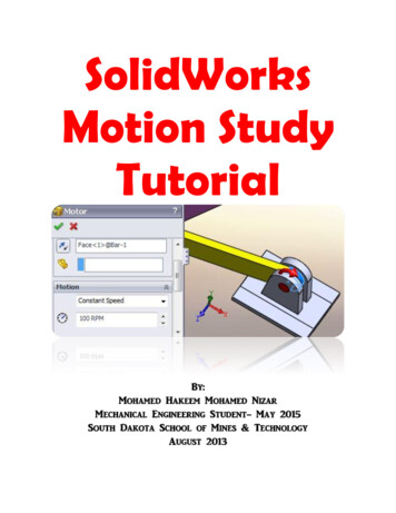
Tzu-Yu WuOpti 521 – Fall 2011Introductory to opto-mechanical engineeringDecember 4th, 2011Introductory Tutorial:SolidWorks Motion and Finite Element Analysis (FEA) Simulation1. Introduction: usage and motivationAfter a design is built, there might be many questions that a designer might need to answer: Will the part fit into the system? Can the part withstand the force before breaking? How would it deform? How does the part move with certain external loads and constrains?These “what if?” questions derive the motivation of simulation. We can bring these questions intoan infinite workspace to virtually test new ideas, develop and optimize designs which would greatlyreduce the expenses and time consumed from product development cycles.FEA simulation can be applied to problems involving vibrations, heat transfer, fluid flow, and manyother areas. This introductory tutorial will focus on motion and stress simulation. Two examples willbe given in Motion simulation. One will be given on FEA. The first example on Motion studyhighlights the key capabilities of Solidworks using simple structures. This tutorial will walk throughthe steps for the first example. The other two examples of each topic demonstrates the simulationsthat I apply on my current research.2A. Motion simulationExample1 : 4 bar linkageHere we will model a 4 bar linkage. The technical drawing is shown in Figure 1.1 with unit in inch.Create each part separately and assemble them as shown in Figure 1.1 by selecting “MakeAssembly from part” under “file”. The bottom bar numbered 3 should be selected first to make theassembly so that it is the fixed link. Each part is assigned “Alloy Steel” as material. (right-clicking“material” in the FeatureManager for each part, and selecting “Edit Material”.)

Figure 1.1 Assembly and dimensions of the partsBefore beginning the simulation, we will set the links to a precise orientation. This will allow us tocompare our results to hand calculations more easily. Add a perpendicular mate between the two facesshown here. Expand the Mates group of the FeatureManager, and right-click on the perpendicular matejust added. Select Suppress.AlignmentThe perpendicular mate aligns the bar 2 at a precise location.Suppressing the perpendicular mate allows us to rotation bar 2freely and unsuppressing it would align it again.MotorActivate Solidworks Motion in add-in. Select the Motor icon.In the PropertyManager, set the velocity to 60 rpm.Click on the front face of the bar 2 to apply the motor, and click the check mark.A one-second simulation will include one full revolution of bar 2 due to 60 rpm.Time settingClick and drag the simulation key from the default five seconds to one second (0:00:01).Frame rateClick the Motion Study Properties Tool.Set the number of frames to 100 (frames per second),and click the check mark.This setting will produce a smooth simulation.Press the Calculator icon to run the simulation.

Results and plotsDisplacementClick the Results and Plots Tools. In the PropertyManager, set the type of the result to Displacement/Velocity/Acceleration: Trace Path. Click on the edge of the top hole of the bar 4.Play back the simulation to see the open hole’s path over the full revolution of bar 2.Figure 1.2 Trace path of holes of bar 4Force and TorqueSelect Results and Plots. In the PropertyManager, specify Forces: Applied Torque: Z Component.Click on the RotaryMotor in the MotionManager to select it, and click the check mark in thePropertyManager.

Exporting dataRight-click in the graph and choose Export CSV. Save the file to a convenient location, and open it inExcel.Plot9Applied Torque3Time (sec)(pound 173591830.003-29.59304906Summary of this exampleIn this example, we simulate the motion of 4 bar linkage with respective to each other.This tutorial shows the following key figures of Motion Simulation in SolidWorks.1. Applying motors to simulate the movement.2. Setting the time flow and frame rate.3. Getting the results and plots and exporting the data.Note: The video can be found in the corresponding PowerPoint file.

2B. Motion simulationExample: Linear and rotational motions of a fiber by a focus motor (actuator)ObjectiveFigure 2.1 Surgical handle for confocal microendoscope. The red highlighted part is our focus of motion simulation.Figure 2.1 shows a microendoscope handle with two linear actuators. One of the actuators servesas a focus motor, which will be our focus. The actuator serves as a focus motor since it moves theimage fiber relative to an objective lens at the distal end. An imaging fiber is connected to theactuator through a rotatable fiber clamp. The rotatable fiber clamp is designed to relieve damagingtwist of the fiber during surgery while still allowing axial translation via the focus motor. The detailsof functionality of this handle are neglected. We will only simulate the motion of the fiber.ComponentsThis model is composed by 4 components- fiber, dumbbell-like holder, connector between fiberand actuator and the actuator. Fiber will be fixed inside the dumbbell holder by injecting epoxy intotwo small holes on the dumbbell holder. Materials are assigned to each part- silica with customizedYoung’s modulous 10.4 Msi, plastic, and stainless steel for fiber, dumbbell holder and connector,and actuator, respectively.Figure 2.2 Components of focusing mechanism on the right hand side and the assembly on the left.

SimulationLinear motor is used for simulating the sinusoidal force (4N) from the actuator from 0 sec to 2, andconstant force from 4 sec to 6 sec. Damper(0.1N) is constantly applied during the whole simulation.Twisting torque on the fiber is simulated by a rotary motor with 30 RPM constant speed from 2 sedto 4 sec. Figure 2.3 shows the simulated loads and figure 2.4 shows the time flow when differentconditions are applied.Figure2.3 Forces and torque are applied at different time points.Figure 2.4 Time flow of the simulationThe results of the simulation can be plotted as a graph or exported as an Excell file. Here we plotangular and linear velocity as demonstrations. Linear velocity reflects the sinusoidal forces during

the first 2 seconds and 0 force from 2seconds to 4 and constant force for the last two seconds.Negative value refers to the direction of movements.Figure 2.5 Results of the simulation.Motion simulation is recorded as a video which can be found in the corresponding PowerPoint file.

3.FEA SimulationBackground understanding:1. What is FEA?FEA performs the stress analysis and also shows critical areas and safety levels at various regions inthe faucet. Based on these results, you can strengthen unsafe regions and remove material fromoverdesigned ones.Figure 3.1 Simulation of deformation and critical regionsParts are simulated by many small elements which share common points called nodes. Thebehavior of these elements is well-known under all possible support and load scenarios. Themotion of each node is fully described by translations in the X, Y, and Z directions, called degrees offreedom (DOFs). Analysis using FEM is called Finite Element Analysis (FEA).Figure3.2 Model subdivided into small pieces (elements)

2. Stress and strainStressStrainYoung’s modulusDeformationFigure 3.3 Explanation and definition of strainFigure 3.4 Plot of Strain v.s. stress

Example: Stress and displacement of a bending fiberFigure 3.5 An articulating tip of a microendoscope handle with an imaging fiber and hypothermic dye line. The redhighlighted region is our simulation focus.System background and motivation of simulationThis microendoscope handle has a flexible catheter which gains more access to imaging organs suchas fallopian tubes during surgeries compared to a rigid device. The articulating distal tip of theinstrument consists of a 2.2 mm diameter bare fiber bundle catheter with automated dye deliverychannel. This simulation is performed to understand the maximum load that the fiber canwithstand before breaking and also the displacement and angles that it can reach within a saferange (safety factor about 3).ModelHyperemic dye tubingApplied force: 1NFixtureImaging fiber - silica with customizedYoung’s modulous 10.4 Msi

ResultsFigure3.6 Stress distribution (on the left) and displacement (on the right)Discussion:The fiber and the dye tubing are bonded together by applying face constraint. Notice that the stressdistribution is different between fiber and dye tubing. It might be due to higher Young’s modulus in thefiber with the same displacement. More cares have to be taken. In this model, many assumptions havebeen make. For example, fiber and dye tubing are constrained together in some degree but not fixedwith each other. However, I bounded them by apply face constraint so that they won’t move relativelyto each other. The edge fixture isn’t true in reality. Material properties of the imaging fiber are criticalfor the simulation.The safety factor can be used to understand the maximum load the part can withstand according to thefollowing equation:Current applied force X Current safetly factor Maximum affordable force.Summary:This tutorial highlights the key functions of SolidWorks Motion and FEA Simulation. The introduction ofFEA theory is briefly given. Detailed tutorial on SolidWorks Motion is given by walking through anexample. Two examples related to imaging fiber motion driven by a linear actuator and fiber bendingare given. There has been much discussion during the past decade over who should be using FEAsoftware. As the software has become easier to use, the potential for misuse has risen. Aninexperienced user can quickly obtain results, but the interpretation of the results requiresknowledge of the applicable engineering theories. In the FEA example, assumptions have beenpointed out that could affect the accuracy of the results.

References:1. Solidworks tutorial and help2. OPTI521 Classnote from Dr Jim Burge3. Tutorials from mcgraw-hill.comUseful learning resources:Complex shapehttp://www.youtube.com/watch?v 3MoowmIKwYQ&feature relatedAssemble study motionhttp://www.youtube.com/watch?v f4BA86PExAQ&feature relatedhttp://www.youtube.com/watch?v cq-kmLC9jkA&feature relatedSpring animationhttp://www.youtube.com/watch?v OYlJT7rhq g&feature relatedMotion simulation with forceshttp://www.youtube.com/watch?v rMeyaO1Kqe0Orally explain rotation movementhttp://www.youtube.com/watch?v efATpeRyLlc&feature relatedGear motion animationhttp://www.youtube.com/watch?v EAGOnKQfJVA&feature relatedMotion study -ball move along a pathhttp://www.youtube.com/watch?v ICwlmlwwCqQ&feature relatedCollision detectionhttp://www.youtube.com/watch?v I xFWKi0xGQ&feature related

This tutorial highlights the key functions of SolidWorks Motion and FEA Simulation. The introduction of FEA theory is briefly given. Detailed tutorial on SolidWorks Motion is given by walking through an example. Two examples related to imaging fiber motion driven by a linear actuator and fiber bending are given. There has been much discussion during the past decade over who should be using FEAFile Size: 718KBPage Count: 12People also search forsolidworks motion tutorial pdfsolidworks motion pdfsolidworks motion simulation pdfsolidworks motion studysolidworks motion study tutorial pdfsolidworks motion tutorial