WIXLIB

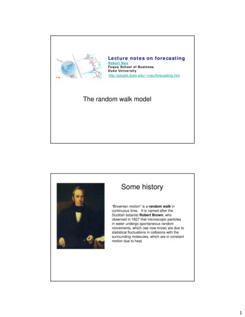
Lecture notes on forecastingRobert NauFuqua School of BusinessDuke Universityhttp://people.duke.edu/ rnau/forecasting.htmThe random walk modelSome history“Brownian motion” is a random walk incontinuous time. It is named after theScottish botanist Robert Brown, whoobserved in 1827 that microscopic particlesin water undergo spontaneous randommovements, which (we now know) are due tostatistical fluctuations in collisions with thesurrounding molecules, which are in constantmotion due to heat.1

http://en.wikipedia.org/wiki/Brownian motionLouis Jean-Baptiste Alphonse Bachelier, aFrench mathematician, was the first person tomodel Brownian motion, as part of his PhD thesis,The Theory of Speculation, published 1900.His thesis, which discussed the use of Brownianmotion to evaluate stock options, is historically thefirst paper to use advanced mathematics in thestudy of finance.2

Five years later, AlbertEinstein (1905)independently discoveredthe same stochasticprocess and applied it inthermodynamics.The mathematical propertiesof a continuous-time randomwalk were later worked outby Norbert Weiner, hencesuch a process is known asa Wiener process,3

Bachelier had derived the price ofan option where the share pricemovement is modelled by a Wienerprocess and derived the price ofwhat is now called a barrier option(namely the option which dependson whether the share price crossesa barrier). Black and Scholes*,following the ideas of Osborne andSamuelson, modelled the shareprice as a stochastic processknown as a geometric Brownianmotion (with drift).In geometric Brownian motion, the natural log of the variable is acontinuous-time random walk with normally distributed steps.*Fischer Black and Myron Scholes, together with Robert Merton, received the Nobel MemorialPrize in economics in 1997, a year before the spectacular collapse of the hedge fund LongTerm Capital Management, on whose board both Scholes and Merton sat.“The market is not a perfectrandom walk. But anysystematic relationships thatexist are so small that theyare not useful for aninvestor The history of stock pricemovements contains nouseful information that willenable an investor tooutperform a buy-and-holdstrategy in managing aportfolio.”(p. 151)4

Don’t take financial advice from babies!The random walk model A time series is a random walk if its period-to-periodchanges are statistically independent & identicallydistributed (“i.i.d.”) In each period it takes an independent random “step” awayfrom its last position If the mean step size is non-zero, it is a random walk “withdrift” (i.e., trend)5

Analogies Random walk: a drunk person staggering left and right withequal probability while moving forward (this was Bachelier’sown example) Random walk with drift: a drunk person with one shoe Continuous random walk (“Brownian motion”): a drunk snailWalking the “drunkard’s walk”6

A random walk with little or no drift often does not look“random”! It may appear to have trends, cycles, “head andshoulders” patterns and other interesting featuresby sheer chance.2520151050050100150200-5-10-15-20-25“It Ain't the Things You Don't Know That Hurt You, It's the Things You Know. That Ain't So!”A related statistical illusion:the “hot hand in basketball” Many basketball players are perceived as “streaky” shooters(e.g., Allen Iverson), but statistical analysis shows that thechance of making a given field goal or free throw is roughlyindependent of what happened on the last few shots:“Chance is a very powerful force in creating streaks" See the Hot Hand in Sports website athttp://thehothand.blogspot.com/7

How to identify a random walk Plot the first difference, i.e., the period-to-period changes, ofthe original time series (Y DIFF1 or DIFF(Y)) If the first difference has constant variance and nosignificant autocorrelations, the original series is a randomwalk (at least locally). If the series is logically bounded above or below or has astable long-run average, then it is not a “true” random walk,but the random walk model may still be appropriate forshort-term forecasting or as a benchmark for comparingfancier models.Relation to mean model If a time series is a random walk, then its first difference isdescribed by the mean model. Thus, you should predict that the next change will equalthe average change. The average change may or may not be zero, dependingon whether there is “drift”.8

Random walk forecast equation In the random walk without drift model, thek-step ahead forecast is the last observed value: In the random walk with drift model, thek-step ahead forecast is the last observed value plus ktimes the estimated drift (trend) per period:Relation to linear trend model A linear trend model assumes that there is a trend line fixed“somewhere in space” around which the data varies in ani.i.d. manner. The fitted trend line always passes through the center ofmass of the data and it regresses toward the X-axis A random-walk-with-drift model also assumes that there is aconstant trend, but it continually “re-anchors” the trend lineon the last observed data point. Confidence intervals for the RW model widen “parabolically”as the forecast horizon increases, but confidence intervalsfor the linear trend model hardly widen at all. Which is morerealistic for your data set?9

Linear trend vs. random walk with driftThe next forecast from arandom walk model willalways be very close to thelast data pointThe trend line doesn’t necessarilypass close to where the data hasbeen lately (at the “business end” ofthe series).A trend line fitted by simple regression is alwaysanchored at the center of mass of the historicaldata and “regresses” toward the X-axis.Linear trend vs. random walk with drift If the growth pattern in the data is irregular or not perfectlylinear, the linear trend model may fit badly near the end ofthe series—which is where the forecasting action occurs! Because the linear trend model anchors the trend line in theexact center of the data, its goodness of fit near the end ofthe series is very sensitive to the amount of history used. Plot of historical RWD forecasts looks like an exact copy ofthe data, but shifted right by 1 period (& perhaps moved up)10

Autocorrelation & the random walk model In a true random walk, there is strong autocorrelation in theoriginal series, but no significant autocorrelation in the firstdifference of the series at any lags. This means there is no pattern in the data except “the changenext period will equal the average change” Hence the random walk model is sometimes called the “naïve”model .but it’s not really naïve! It says you can’t do better than this,and it has profound and financially important implications forwidths of confidence intervals for forecasts at horizons of morethan one period ahead.Geometric random walk If the log of a series is a random walk, the original series is ageometric random walk. Recall that the change in the natural log is (approximately) thepercentage change between periods :LN Yt LN Yt 1 Yt / Yt 1 1LN Yt / Yt 1Yt Yt 1 / Yt 1 ! Hence, in a geometric random walk, the series takes randomsteps in (roughly) percentage termsPercentage change is a more familiar and easy-to-think-aboutconcept, but change-in-the-natural-log is theoretically the right way tomeasure relative changes when exponential growth is occurring orwhen small changes are compounded over many periods.11

Diff-log vs. percent change% change in �2%0%2%5%10%20%30%40%50%90%100%diff‐log of 2620.3360.4050.6420.693diff‐log of 3000.4000.5000.6000.700% change in %‐82.2%‐101.4%Almost thesame up toaround 10%,and pretty closeup to 20%,Diff-log of X isX LN DIFF1 inRegressIt andDIFF(LOG(X)) inStatgraphics% change of X from period t to period t 1 is Xt Xt‐1 /Xt‐1Diff-log of X from period t to period t 1 is LN Xt LN Xt‐1Geometric random walk forecast equation In log units:1 i.e., LN Y is predicted to grow linearly with trend r In unlogged (original) units:1 i.e., Y is predicted to compound at rate r12

Best example: stock prices The geometric random walk is the “default” model for stockprices and many other financial assets for whichspeculative markets exist First proposed by Bachelier in 1900, it became the basis forthe Black-Scholes options pricing model 70 years later. This means it is hard to beat the market by technicalanalysis (“charting”). or by fitting regression models to monthly, weekly, oreven daily data.Why should stock prices behave like ageometric random walk? If everyone could predict that the stock market will go upmore than average tomorrow, it would have already gone uptoday, hence future returns are independent of past returns(and other public information) in an efficient market. Investors generally think in terms of percentage changes instock values when responding to informational events(earnings announcements, interest hikes, etc.), hencevolatility is fairly constant in percentage terms. Remarkably, the average volatility has been consistent inpercentage terms over the last century.13

Forecasting from the GRW model First apply the standard RW model to the logged series toobtain forecasts and confidence intervals in logged units Then “unlog” them (apply the “EXP” function) to obtainforecasts and confidence intervals in original units. The forecasting procedure in Statgraphics does all thisautomatically when you specify a random walk model inconjunction with with a log transformation.ExampleOriginal series shows erraticbehavior, strong positiveautocorrelation, peaks andvalleys, exponential growthThe heights of the bars are theautocorrelations. Here theautocorrelations are all close to 1because the series tends to remainon the same side of its samplemean for long periods.14

ExampleA natural log transformationlinearizes the long-run growth.Slope of line drawn between1st and last points is theaverage percent growth.ExampleAfter a diff-log transformation,the variance is roughly constant(over the long run, at least) andautocorrelations are allinsignificant, the signature of ageometric random walk15

Forecasting from the random walk model The forecasts from the random walk model areextrapolated as a straight line extending from the lastobserved data point. In a random walk without drift, the line is horizontal. In a random walk with drift, it has a non-zero slope. Drift estimation is hard unless the sample size is hugeand/or you have a theoretical basis for determining it fromother data (as in the CAPM) If the drift is estimated from the sample, the forecasts arethe extrapolation of a line through the 1st and last points!Standard errors of forecasts The standard error of a one-step-ahead RW forecast isthe sample standard deviation of the differenced seriesmultiplied by SQRT(1 1/(n-1)) where n is the sample size.– Same as the standard error of the forecast whenapplying the mean model to the differenced series,whose length is n-1 rather than n The standard error of a k-step-ahead RW forecast is equalto the standard error of a one-step-ahead RW forecastmultiplied by a growth factor of SQRT(k)– Why .?16