WIXLIB

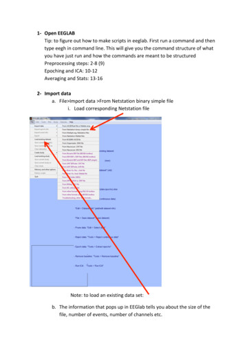
1- Open EEGLABTip: to figure out how to make scripts in eeglab. First run a command and thentype eegh in command line. This will give you the command structure of whatyou have just run and how the commands are meant to be structuredPreprocessing steps: 2-8 (9)Epoching and ICA: 10-12Averaging and Stats: 13-162- Import dataa. File Import data From Netstation binary simple filei. Load corresponding Netstation fileNote: to load an existing data set:b. The information that pops up in EEGlab tells you about the size of thefile, number of events, number of channels etc.

c. Save data so it is easier to have the data stored as a .set file in eeglab –to reopend. SAVE (“ss expt name scroll”)3- Plot and remove artefacts (optional)a. It is sometimes a good idea to scroll through the entire raw data – tomake sure everything went ok during recording. While this can be a bittime consuming, it will give you more familiarity as to whether thereare any odd channels that may need interpolating later on, or largeartefacts that should be removed from any further analysis.b. To plot: Plot Channel data (scroll)c. Remove DC offset: Display Remove DC offset

Settings: Time range to display, Number of channels,EventNumberd. To move through the plot use the arrow keyse. SAVE (“ss expt name scroll”)Scale

4- Extract triggers (if applicable)a. If you want to remove triggers (i.e. remove incorrect trials fromanalysis), or insert different labels for triggers then it is easier to do thisat this early stage.b. To extract triggers (EEG.event) – then run a program selecting thetriggers you want – the important information to keep is the type andlatency of the trigger.c. Add event triggers into file: file importeventfile from matlab array:type in “EEG.event” into arrayd. SAVE (“ss expt name trig”)5- Import channel location filea. Need to insert channel information. This is stored in a text documentwith electrode label and x/y co-ordinates (location) of the electrodes(e.g. Cz is 0,0)b. Edit Channel locationsi. Make sure BESA spherical file is selected Press Okc. Read locations select: GSN124 plus.loc

i. Select: autodetect Press OKd. Press Ok on Edit chan info windowe. In data set file – Channel Locations should now have changed to a “yes”f. SAVE (“ss expt name chan”)6- Filters (use FIR)a. Tools Filter the data Basic (FIR)

b. Apply high pass filter first (e.g. 0.01Hz)c. Once the data has been high-pass filtered

d. Apply low pass filter next (e.g. 80Hz)e. Note: filtering can distort data or clean it up, Luck has a great chapteron how and when to use filtersf. SAVE (“ss expt name filt”)7- Identify Bad Channelsa. Tools Automatic channel rejection]b. The Output of this can be copied into an Excel file and saved.c. Highlight any channel labelled as bad and take note of the electrodenumber

d. OR: Edit Select Data Channel Data (I AM UP TO HERE!!)8- Interpolation (as a preprocessing step - do this once you have run through 1to 12 once) Note: you can also interpolate after epoch and ica’ing but willhave to re-reference after ICA.a. When channels are bad/noisy/flat and are contributing to epochrejection then you need to interpolate the electrode. Interpolationtakes an average of the signal from surrounding electrodes so that the

bad signal becomes an interpolation of the signal from the surroundingelectrodesb. If this is done before the ICA (i.e. before epoch extraction) the dataentered into the ICA is cleanc. Tools Interpolate electrodesd. Select from data channelsi. pick channels you want to interpolateSelect data channelsThis needs to be sphericale. Interpolation method: spherical methodf. SAVE (“ss expt name interp”)9- Rereferencea. Tools Re-reference

b. For an average reference:i. Click “compute average reference”ii. In box for “add current reference channel back to the data” typein your reference channel (e.g. Cz)c. For a channel reference (e.g mastoids: TP9 and TP10):i. Click “re-reference data to channel” and select channels youwant to reference toii. In box for “add current reference channel back to the data” typein your reference channel (e.g. Cz)d. SAVE (“ss expt name reref”)10- Extract data epochsa. Once pre-processed data (Steps 1-9), use the final pre-processed data(“ss seq omit interp”) to extract data epochs. Need to decide the

triggers (time locking events), the size of the epoch window whichincludes pre-stimulus and post-stimulus (in seconds e.g. -.5 to 1), thebaseline (in milliseconds e.g. -100 to 0)b. Tools Extract EpochsSelect Epochs – by pressing .Epoch time window (in secs)i. Time-locking event: select triggersii. Epoch limits: epoch time window [start time, end time]iii. Save dataset (“ss expt name epoch name”)iv. Popup: baseline removalBaseline window(in ms e.g -100to 0)

1. Baseline latency range [start time for baseline, end timefor baseline] (note in ms) Ok2. SAVE: File save current data set(“ss expt name epoch name base”)c. MAKE SURE YOU SAVE THE EPOCHED DATA – and that you remove thebaseline – as this will really mess up your trials marked for rejections.d. If you are looking at different epochs e.g. pre-action activity vs stimuluslocked ERP then need to create different epochs for each.11- Run ICA for blink correctiona. In order to remove blink artefacts an ICA is run on the epoched datab. Tools Run ICAi. This will take a while – it can be from an hour to a few hoursdepending on the size of your epoched datac. SAVE (“ss expt name epoch name ica”). Make sure you save this file– as you don’t want to redo the ica because you forgot to save it.d. To look at the ICAs: Tools Reject Data using ICA reject components bymap – should pop up a window that asks how many components toplotIC1 – maybeblinkIC2 – may beeyemovementse. Select component with blinks in them – check the power spectrum (andeeglab wiki for what to look at)

Frontal activity onlyBoth frontal andoccipital activityEvents peakat same timeacross epochsEvents spreadacross epochsPower log showsno real peaksA BlinkNot a Blinkf. Tools Remove components (this is to see if the data is correcting theblink)i. Enter component to remove from data: blink ICA no. (e.g 1)ii. Leave “component to overwrite” blankiii. When “confirmation” dialog box opens click on “plot singletrials”iv. The red line in the plots is your “corrected” raw trace and theblack line is your previous epochs – for blink correction thereshould be a big difference in blinks between red and black lines.

Black line: original traceRed Line: corrected traceIf blink: the correctedtrace affects mainlyfrontal channelsIf blink: the correctedtrace should flattensignal of the blinkv. If you want to accept for rejection then click ACCEPT if not thenclick CANCELvi. SAVE the new file as (“ss expt name epoch name bc”)

g. Save the component numbers that have been removed in excel or anotepad document.12- Reject Data Epochsa. To select data epochs for averaging and analysis – need to excludeepochs based on a specific criteria (such as extreme values or low signaldrift or sudden gradient changes). Only epochs that meet this criteriawill be included in analysis. This is an example for extreme values.b. Tools Reject data epochs reject extreme valuesi. Upper/lower limits ( 120/-120) (or 100 depending on how strictyou are).ii. Start time/End time: specify the window you want artefactrejection to take place. Generally use the start of the epoch tothe end of the epoch, but sometimes you may want a largeepoch but only want artefact rejection to happen over a smallerwindow.iii. Display with previously marked rejections and Reject markedtrials: keep at default “No”Upper andLower limitsStart EpochEnd Epochc. Popup data plot: This will then highlight the epochs that have extremevalues in them

Electrode exceedingthresholdi. Similar to blink correction – a trace in an electrode that is redmeans it has exceeded your criteriaii. You can visually inspect and then decide whether to accept themor not.iii. If you think the epoch is ok – then click on it and it should not behighlighted anymore – then click update marks.iv. If the same electrode is contributing to a lot of rejected epochsthen you may want to look into interpolating that channel (youwill need to go back to the Interpolation step)v. Can determine if a channel is contributing to rejection thresholdand decide to interpolate (see 9. Interpolation).1. Epochs that are going to be rejected are in workspace asEEG.reject.rejthreshE (channel x epoch matrix).2. If there is a “1” in a cell it means it is tagged for rejection3. Sort through each channel (row) to determine how manyepochs are marked for rejection4. Generally if there is at least 20-25% of epochs rejected –then the channel needs interpolating5. EEG lab allows interpolation of a channel at this point too(refer to 8 on how to interpolate a channel).

6. If interpolating at this point then must apply the averagereference after interpolation and not at the preprocessingstepd. Tools Reject data epochs reject marked epochs (remember once youhave marked epochs to reject doesn’t mean that they have beenrejected) Make sure you do this step.e. SAVE (“ss expt name epoch name rej”)f. Take note of the no. of trials rejected – for erps – ideally need at least80 trials in each condition (or over 75 to 80% of all trials accepted)–anything less than participant should be rejected from further analysisfor failing to reach threshold13- Selecting Data Epochs (Conditions)a. For each ica corrected/artefact rejected epoch{ss expt name epoch name rej } need to create separate conditionsfor each subjectb. Edit Select Epochs/Eventsc. In the dialog box for select the event click on type “ ” and select thecondition you want to use (you will create one of these condition filesfor each condition)Only selectone at a timeMake sure thisis selected

d. Need to select (i.e. click) remove epochs not referenced by anyselected event – OKe. Click OK for warning dialogue box.f. Name it something different– and save all of these files to a folderwithin your epoched data folder. Again change the name for each file.SAVE (“ss expt name epoch name condition name“).g. Important: Note down the no. of epochs that are now included in thatevent (as this may be important for subject rejection etc.)h. Redo this for each condition/event you want to look at - make sure yougo back to the set file containing all events and not the condition files.14- Compare Events for One Subject using Plotsa. Load condition datasets (you will be using the dataset number in theeeglab dialog box that has been assigned to these files)b. Plot sum/compare erpsdifferenceaverageData sets to plotTo create SD ofaverageSingle trials/each datasetTo compareconditions /datasetsAlpha criteriaNegative plotted upc. In the blank white spaces enter in the data sets you want to plot e.g. 124d. If want to average together then click “avg”e. If don’t want the average across the entered conditions then click “allerps”f. If you want to compare between conditions enter one set of data setsin “datasets to average” then put the comparison data sets into