Transcription
Python tutorial netcdfSeptember 10, 2018In [1]: %matplotlib inlineReading Scientific Datasets in Python Todd Spindler IMSG at NCEP/EMC Verification PostProcessing Product Generation Branch Learn scientific data visualization in three easy* lessons!; *and many more perhaps not-quite-so-easy lessons.Just an FYI before we begin This entire presentation was created using Python 3 and Jupyter Notebooks All three example notebooks and the data sets are available from our web site:– http://polar.ncep.noaa.gov/ngmmf python Feel free to download them and play with the notebooksThree commonly used binary dataset formats in use at EMC are (in no particular order): NetCDF (Network Common Data Format) GRIB (GRIdded Binary or General Regularly-distributed Information in Binary form) BUFR (Binary Universal Form for the Representation of meteorological data)0.0.1 Example 1: Reading a NetCDF data setNetCDF can be read with any of the following libraries: - netCDF4-python xarray PyNIOIn this example we’ll use xarray to read a Global RTOFS NetCDF dataset, plot a parameter(SST), and select a subregion.The xarray library can be installed via pip, conda (or whatever package manager comes withyour Python installation), or distutils (python setup.py). Begin by importing the required libraries.In [2]: importimportimportimportmatplotlib.pyplot as plt# standard graphics libraryxarraycartopy.crs as ccrs# cartographic coordinate reference systemcartopy.feature as cfeature # features such as land, borders, coastlines1
Open the file as an xarray Dataset and display the metadata.In [3]: dataset xarray.open dataset('rtofs glo 2ds n000 daily prog.nc',decode times True) decode times True will automatically decode the datetime values from NetCDF conventionto Python datetime objects Note that this reads a local data set, but you can replace the filename with the URL of thecorresponding NOMADS OpenDAP data set and continue without further changes.In [4]: datasetOut[4]: xarray.Dataset Dimensions:Coordinates:* MTDate* Layer* Y* XLatitudeLongitudeData variables:u velocityv velocitysstssslayer urce:experiment:history:(Layer: 1, MT: 1, X: 4500, Y: 3298)(MT) datetime64[ns] 2018-08-26(MT) float64 .(Layer) int32 1(Y) int32 1 2 3 4 5 6 7 8 9 10 11 12 13 14 15 16 17 18 19 .(X) int32 1 2 3 4 5 6 7 8 9 10 11 12 13 14 15 16 17 18 19 .(Y, X) float32 .(Y, X) float32 .(MT,(MT,(MT,(MT,(MT,Layer, Y, X) float32 .Layer, Y, X) float32 .Y, X) float32 .Y, X) float32 .Layer, Y, X) float32 .CF-1.0HYCOM ATLb2.00National Centers for Environmental PredictionHYCOM archive file09.2archv2ncdf2d There’s an extra Date field. Since it’s not needed, here’s how to get rid of it.In [5]: dataset dataset.drop('Date') You can also use the python delete command: del dataset['Date'] There’s a quirk in the Global RTOFS datasets -- the bottom row of the longitude field isunused by the model and is filled with junk data. I’ll use array subsetting to get rid of it, and save just the SST parameter to a separate DataArray.In [6]: sst dataset.sst[0,0:-1,:]# this can be shortened to [0,:-1,]2
Note that subsetting an xarray parameter will also subset the associated coordinates at thesame time.In [7]: sstOut[7]: xarray.DataArray 'sst' (Y: 3297, X: 4500) [14836500 values with dtype float32]Coordinates:MTdatetime64[ns] 2018-08-26* Y(Y) int32 1 2 3 4 5 6 7 8 9 10 11 12 13 14 15 16 17 18 19 20 .* X(X) int32 1 2 3 4 5 6 7 8 9 10 11 12 13 14 15 16 17 18 19 20 .Latitude(Y, X) float32 .Longitude (Y, X) float32 .Attributes:standard name: sea surface temperatureunits:degCvalid range:[-2.1907086 34.93205 ]long name:sea surf. temp.[09.2H] For a quick look at the raw data array, use matplotlib’s imshow function to display the SSTparameter as an image.In [8]: plt.figure(dpi 100)# open a new figure window and set the resolutionplt.imshow(sst,cmap 'gist ncar'); This is how the model data is stored in the array. The Latitude array is similarly upsidedown.3
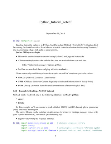
Also note that the longitude values are a bit odd.In [9]: print(sst.Longitude.min().data, sst.Longitude.max().data)74.1199951171875 434.1199951171875 In fact, the whole model grid is pretty weird. It’s called a tripolar grid. Now set up the figure and plot the sst field in a Mercator projection, using Cartopy to handlethe projection details and letting xarray decide how to plot the data. The default for 2-Dplotting is pcolormesh(). Xarray is very smart and will try to use a diverging (bicolor) colormap if the data valuesstraddle zero. You override this by specifying the colormap with cmap and the vmin , vmax values foryour data.In [10]: plt.figure(dpi 100)ax plt.axes(projection ccrs.Mercator())ax.add feature(cfeature.LAND)ax.coastlines()gl ax.gridlines(draw labels True)gl.xlabels top Falsegl.ylabels right False####fill in the land areasuse the default low-resolution coastlinedefault is to label all axes.turn off two of them.sst.plot(x 'Longitude',y 'Latitude',cmap 'gist ncar',vmin sst.min(),vmax sst.max(),transform ccrs.PlateCarree());4
Now let’s concentrate on the waters around Hawaii (lat: 17 to 24, lon: -163 to -153) RTOFS longitudes are defined as 74-430, so we need to convert the -163 and -153 values bycomputing modulo 360. Use the object.where() method with the lat/lon limits.In [11]: hawaii sst.where((sst.Longitude -163%360) & (sst.Longitude -153%360) &(sst.Latitude 17) & (sst.Latitude 24), drop True) Note the drop True option, which instructs the .where() method to subset the data. Otherwise it will retain the full array size and simply mask out the unwanted data. As before, let’s plot the SST in a Mercator projection, but use a high-resolution coastline. Since the water around Hawaii is warm I don’t have to specify the colormap limits.In [12]: plt.figure(dpi 100)ax plt.axes(projection ccrs.Mercator())ax.add feature(cfeature.LAND)ax.add feature(cfeature.GSHHSFeature()) # use a high-resolution GSHHS coastlinegl ax.gridlines(draw labels True)gl.xlabels top Falsegl.ylabels right Falsehawaii.plot.contourf(x 'Longitude',y 'Latitude',levels 20,cmap 'gist ncar',add colorbar True,transform ccrs.PlateCarree());5
0.1Next Example -- Reading a GRIB file6
your Python installation), or distutils (python setup.py). Begin by importing the required libraries. In [2]: import matplotlib.pyplot as plt # standard graphics library import xarray import cartopy.crs as ccrs # cartographic coordinate reference system import cartopy.feature a