Transcription
3Polynomial Approximation,Interpolation, andOrthogonal Polynomials In the last chapter we saw that the eigen-equation for a matrix wasa polynomial whose roots were the eigenvalues of the matrix. However, polynomials play a much larger rolein numerical analysis than providing just eigenvalues. Indeed, the foundation of most numerical analysismethods rests on the understanding of polynomials. As we shall see, numerical methods are usually tailoredto produce exact answers for polynomials. Thus, if the solution to a problem is a polynomial, it is oftenpossible to find a method of analysis, which has zero formal truncation error. So the extent to which aproblem's solution resembles a polynomial will generally determine the accuracy of the solution. Thereforewe shall spend some time understanding polynomials themselves so that we may better understand themethods that rely on them.55
Numerical Methods and Data Analysis3.1Polynomials and Their RootsWhen the term polynomial is mentioned, one generally thinks of a function made up of a sum ofterms of the form ai xi. However, it is possible to have a much broader definition where instead of the simplefunction xi we may use any general function φi(x) so that a general definition of a polynomial would havethe formnP( x ) a i φ i ( x ) .(3.1.1)i 0Here the quantity n is known as the degree of the polynomial and is usually one less than the number ofterms in the polynomial. While most of what we develop in this chapter will be correct for generalpolynomials such as those in equation (3.1.1), we will use the more common representation of thepolynomial so thati(3.1.2)φi(x) x .Thus the common form for a polynomial would beP(x) a0 a1x a2x2 anxn .(3.1.3)Familiar as this form may be, it is not the most convenient form for evaluating the polynomial. Consider thelast term in equation (3.1.3). It will take n 1 multiplications to evaluate that term alone and n multiplicationsfor the next lowest order term. If one sums the series, it is clear that it will take (n 1)n/2 multiplications andn additions to evaluate P(x). However, if we write equation (3.1.3) asP( x ) a 0 (a 1 L (a n 1 a n x ) x ) x L) x ,(3.1.4)then, while there are still n additions required for the evaluation of P(x), the number of multiplications hasbeen reduced to n. Since the time required for a computer to carry out a multiplication is usually an order ofmagnitude greater than that required for addition, equation (3.1.4) is a considerably more efficient way toevaluate P(x) than the standard form given by equation (3.1.3). Equation (3.1.4) is sometimes called the"factored form" of the polynomial and can be immediately written down for any polynomial. However, thereis another way of representing the polynomial in terms of factors, namelyP( x ) a n ( x x 1 )( x x 2 )( x x 3 ) L ( x x n ) .(3.1.5)Here the last n coefficients of the polynomial have been replaced by n quantities known as the roots of thepolynomial. It is important to note that, in general, there are (n 1) parameters specifying a polynomial ofdegree n. These parameters can be either the (n 1) coefficients or the n roots and a multiplicative scale factoran. In order to fully specify a polynomial this many parameters must be specified. We shall see that thisrequirement sets constraints for interpolation.The n quantities known as the roots are not related to the coefficients in a simple way. Indeed, it isnot obvious that the polynomial should be able to be written in the form of equation (3.1.5). The fact that a56
3 - Polynomial Approximationpolynomial of degree n has exactly n such roots is known as the fundamental theorem of algebra and itsproof is not simple. As we shall see, simply finding the roots is not simple and constitutes one of the moredifficult problems in numerical analysis. Since the roots may be either real or complex, the most generalapproach will have to utilize complex arithmetic. Some polynomials may have multiple roots (i.e. more thanone root with the same numerical value). This causes trouble for some root finding methods. In general, it isuseful to remove a root (or a pair if they are complex) once it is found thereby reducing the polynomial to alower degree. Once it has been reduced to a quadratic or even a cubic, the analytic formulae for these rootsmaybe used. There is an analytic form for the general solution of a quartic (i.e. polynomial of 4th degree),but it is so cumbersome that it is rarely used. Since it has been shown that there is no general form for theroots of polynomials of degree 5 or higher, one will usually have to resort to numerical methods in order tofind the roots of such polynomials. The absence of a general scheme for finding the roots in terms of thecoefficients means that we shall have to learn as much about the polynomial as possible before looking forthe roots.a.Some Constraints on the Roots of PolynomialsThis subject has been studied by some of the greatest mathematical minds of the last severalcenturies and there are numerous theorems that can be helpful in describing the roots. For example, if we remultiply equation (3.1.5) the coefficient of xn-1 is just an times the negative summation of the roots so thatnan-1 an Σ xi .(3.1.6)a n 2 a n x i x j .(3.1.7)i 1In a similar manner we find thati jjWe will see that it is possible to use these relations to obtain estimates of the magnitude of the roots. Inaddition, the magnitude of the roots is bounded by(a 1) x j ( a max 1) . 1max(3.1.8)Finally there is Descarte's rule of signs which we all learned at one time but usually forgot. If wereverse the order of equation (3.1.3) so that the terms appear in descending powers of x asP( x ) a n x n a n 1 x n 1 a n 2 x n 2 L a 0 ,(3.1.9)then any change of sign between two successive terms is called a variation in sign. Coefficients that are zeroare ignored. With that definition of a sign variation we can state Descarte's rule of signs asThe number of positive roots of P(x) 0 cannot exceed the number of variations of sign inP(x) and, in any case, differs from the number of variations by an even integer.A useful and easily proved corollary to this isThe number of negative roots of P(x) 0 cannot exceed the number of variations in sign inP(-x) and, in any case, differs from the number of variations by an even integer.57
Numerical Methods and Data AnalysisThe phrasing concerning the "even integer" results from the possibility of the existence of complex roots,which occur, in pairs (providing the coefficients are real) where one is the complex conjugate of the other.With these tools, it is often possible to say a good deal about the properties of the roots of the polynomial inquestion. Since most of the methods for finding roots are sequential and require the removal of the rootsleading to a new polynomial of lower degree, we should say something about how this is accomplished.b.Synthetic DivisionIf we wish to remove a factor from a polynomial we may proceed as if we were doing longdivision with the added proviso that we keep track of the appropriate powers of x. Thus if (x-r) is to befactored out of P(x) we could proceed in exactly the same fashion as long division. Consider the specificcase where r 2 andP(x) x4 3x3 17x2 6x 18 .(3.1.10)The long division would then look likex 3 5x 2 7 x 11( x 2) x 4 3x 3 17 x 2 3x 18x 4 2x 35x 3 17 x 25x 3 10 x 2 7 x 2 3x 7x 2 14 x 11x 18 11x 22 40 .(3.1.11)Thus we can write P(x) asP(x) (x-2)(x3 5x2-7x-11) 40/(x-2) ,(3.1.12)P(x) (x-r)Q(x) R .(3.1.13)P(r) R .(3.1.14)or in general asSo if we evaluate the polynomial for x r we get58
3 - Polynomial ApproximationNow if R(r) is zero, then r is a root by definition. Indeed, one method for improving roots is to carry outrepeated division, varying r until the remainder R is acceptably close to zero. A cursory inspection of thelong division expression (3.1.11) shows that much more is being written down than is necessary. In order forthe division to proceed in an orderly fashion, there is no freedom in what is to be done with the leadcoefficients of the largest powers of x. Indeed, the coefficients of the resultant polynomial Q(x) are repeatedbelow. Also, when searching for a root, the lead coefficient of x in the divisor is always one and thereforeneed not be written down. Thus if we write down only the coefficients and r-value for the division process,we can compress the notation so thatr 2 1 3 17 3 18 P( x ) 2 10 14 22Q( x ) 1 5 7 11 40 R . (3.1.15)This shorthand form of keeping track of the division is known as synthetic division. Even this notation canbe formulated in terms of a recursive procedure. If we let the coefficients of the quotient polynomial Q(x) bebi so that(3.1.16)Q(x) b0 b1x b2x2 bn-1xn-1 ,then the process of finding the bi's in terms of the coefficients ai of the original polynomial P(x) can bewritten asb n 1 a nb i 1 rb i a iR b 1 i 0L n 1 . (3.1.17)Here the remainder R is given by b-1 and should it be zero, then r is a root. Therefore, once a root has beenfound, it can be removed by synthetic division leading to an new polynomial Q(x). One can then begin againto find the roots of Q(x) until the original polynomial has been reduced to a cubic or less. Because of thecomplexity of the general cubic, one usually uses the quadratic formula. However, even here Press et al1suggest caution and recommend the use of both forms of the formula, namely b b 2 4acx 2a2cx b b 2 4ac . (3.1.18)Should a or c be small the discriminate will be nearly the same as b and the resultant solution will sufferfrom round-off error. They suggest the following simple solution to this problem. Defineq [b sgn(b) b 2 4ac ] / 2 .(3.1.19)Then the two roots will be given by59
Numerical Methods and Data Analysisx q/a .x c/q (3.1.20)Let us see how one might analyze our specific polynomial in equation (3.1.10). Descartes’ rule ofsigns for P(x) tells us that we will have no more than three real positive roots while for P(-x) it states that wewill have no more than one real negative root. The degree of the polynomial itself indicates that there will befour roots in all. When the coefficients of a polynomial are integer, it is tempting to look for integer roots. Alittle exploring with synthetic division shows that we can find two roots so thatP(x) (x-3)(x 6)(x2 1) ,(3.1.21)and clearly the last two roots are complex. For polynomials with real coefficients, one can even use syntheticdivision to remove complex roots. Since the roots will appear in conjugate pairs, simply form the quadraticpolynomial(x-r)(x-r*) x2 (r r*)x r r* ,(3.1.22)which will have real coefficients as the imaginary part of r cancels out of (r r*) and rr* is real by definition.One then uses synthetic division to divide out the quadratic form of equation (3.1.22). A general recurrencerelation similar to equation (3.1.17) can be developed for the purposes of machine computation.Normally the coefficients of interesting polynomials are not integers and the roots are not simplenumbers. Therefore the synthetic division will have a certain round off error so that R(r) will not be zero.This points out one of the greatest difficulties to be encountered in finding the roots of a polynomial. Theround off error in R(r) accumulates from root to root and will generally depend on the order in which theroots are found. Thus the final quadratic polynomial that yields the last two roots may be significantlydifferent than the correct polynomial that would result in the absence of round off error. One may get afeeling for the extent of this problem by redoing the calculation but finding the roots in a different order. Ifthe values are independent of the order in which they are found, then they are probably accurate. If not, thenthey are not.c.The Graffe Root-Squaring ProcessWe discuss this process not so much for its practical utility as to show the efficacy of theconstraints given in equations (3.1.6,7). Consider evaluating a polynomial for values of x xi where xi arethe roots so thatP( x i ) a i x ij a 2 k x i2 k a 2 k 1 x i2 k 1 .(3.1.23) kjWe may separate the terms of the polynomial into even and odd powers of x and since P(xi) 0, we mayarrange the odd powers so that they are all on one side of the equation as22 2 k 1 2k a 2 k x i a 2 k 1 x i . k k 60(3.1.24)
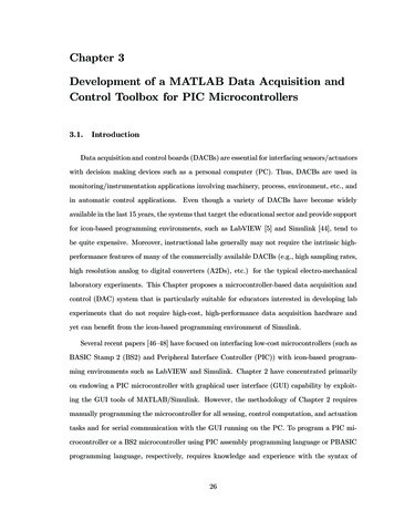
3 - Polynomial ApproximationSquaring both sides produces exponents with even powers and a polynomial with new coefficients aiand having the formS( x ) a (np ) x 2 pn a (np ) x 2 pn 2 L a (0p )(3.1.25).(p)These new coefficients can be generated by the recurrence relation fromn 1 a i( p 1) 2a (np ) a (2pl) 2 a (kp ) a (2pl) k ( 1) l (a 1( p ) ) 2 k l 1 .( p) a i 0, i n (3.1.26)If we continue to repeat this process it is clear that the largest root will dominate the sum in equation (3.1.6)so thatn ( p) p Lim x i2 p Lim a n 1 ( p ) .x 2maxp p an i 1(3.1.27)Since the product of the largest two roots will dominate the sums of equation (3.1.7), we may generalize theresult of eq (3.1.27) so that each root will be given by (p) x i2 p Lim a i 1 ( p ) p an .(3.1.28)While this method will in principle yield all the roots of the polynomial, the coefficients grow so fast thatroundoff error quickly begins to dominate the polynomial. However, in some instance it may yieldapproximate roots that will suffice for initial guesses required by more sophisticated methods. Impressive asthis method is theoretically, it is rarely used. While the algorithm is reasonably simple, the large number ofdigits required by even a few steps makes the programming of the method exceedingly difficult.d.Iterative MethodsMost of the standard algorithms used to find the roots of polynomials scan the polynomialin an orderly fashion searching for the root. Any such scheme requires an initial guess, a method forpredicting a better guess, and a system for deciding when a root has been found. It is possible to cast anysuch method in the form of a fixed-point iterative function such as was discussed in section 2.3d. Methodshaving this form are legion so we will discuss only the simplest and most widely used. Putting aside theproblem of establishing the initial guess, we will turn to the central problem of predicting an improved valuefor the root. Consider the simple case of a polynomial with real roots and having a value P(x k) for somevalue of the independent variable x k (see Figure 3.1).61
Numerical Methods and Data AnalysisFigure 3.1 depicts a typical polynomial with real roots. Construct the tangent to the curveat the point xk and extend this tangent to the x-axis. The crossing point xk 1 represents animproved value for the root in the Newton-Raphson algorithm. The point xk-1 can be used toconstruct a secant providing a second method for finding an improved value of x.Many iterative techniques use a straight line extension of the function P(x) to the x-axis as a meansof determining an improved value for x. In the case where the straight-line approximation to the function isobtained from the local tangent to the curve at the point xk, we call the method the Newton-Raphson method.We can cast this in the form of a fixed-point iterative function since we are looking for the place where P(x) 0. In order to find the iterative function that will accomplish this let us assume that an improved value ofthe root x(k) will be given byx(k 1) x(k) [x(k 1)-x(k)] x(k) x(k) .(3.1.29)Now since we are approximating the function locally by a straight line, we may write . β P[ x ( k ) ] αx ( k ) βP[ x ( k 1) ] αx ( k 1)(3.1.30)Subtracting these two equations we getP[x(k)] α[x(k) x(k 1)] α x(k) .62(3.1.31)
3 - Polynomial ApproximationHowever the slope of the tangent line α is given by the derivative so thatα dP[x(k)]/dx .(3.1.32)Thus the Newton-Raphson iteration scheme can be written asx(k 1) x(k) P[x(k)]/P'[x(k)] .(3.1.33)By comparing equation (3.1.33) to equation (2.3.18) it is clear that the fixed-point iterative function forNewton-Raphson iteration isΦ(x) x P(x)/P'(x) .(3.1.34)We can also apply the convergence criterion given by equation (2.3.20) and find that the necessaryand sufficient condition for the convergence of the Newton-Raphson iteration scheme isP( x )P" ( x ) 1 , x ε x ( k ) x x 02[P' ( x )].(3.1.35)Since this involves only one more derivative than is required for the implementation of the scheme, itprovides a quite reasonable convergence criterion and it should be used in conjunction with the iterationscheme.The Newton-Raphson iteration scheme is far more general than is implied by its use in polynomialroot finding. Indeed, many non-linear equations can be dealt with by means of equations (3.1.34, 35). Fromequation (3.1.33), it is clear that the scheme will yield 'exact' answers for first degree polynomials or straightlines. Thus we can expect that the error at any step will depend on [ x(k)]2. Such schemes are said to besecond order schemes and converge quite rapidly. In general, if the error at any step can be written asE(x) K ( x)n ,(3.1.36)where K is approximately constant throughout the range of approximation, the approximation scheme is saidto be of (order) O( x)n. It is also clear that problems can occur for this method in the event that the root ofinterest is a multiple root. Any multiple root of P(x) will also be a root of P'(x). Geometrically this impliesthat the root will occur at a point where the polynomial becomes tangent to the x-axis. Since the denominatorof equation (3.1.35) will approach zero at least quadratically while the numerator may approach zero linearlyin the vicinity of the root(s), it is unlikely that the convergence criterion will be met. In practice, the shallowslope of the tangent will cause a large correction to x(k) moving the iteration scheme far from the root.A modest variation of this approach yields a rather more stable iteration scheme. If instead of usingthe local value of the derivative to obtain the slope of our approximating line, we use a prior point from theiteration sequence, we can construct a secant through the prior point and the present point instead of the localtangent. The straight line approximation through these two points will have the form , β P[ x ( k ) ] αx ( k ) βP[ x ( k 1) ] αx ( k 1)(3.1.37)which, in the same manner as was done with equation (3.1.30) yields a value for the slope of the line of63
Numerical Methods and Data Analysisα P[ x ( k ) ] P[ x ( k 1) ].x ( k ) x ( k 1)So the iterative form of the secant iteration scheme isx ( k 1) x ( k ) [P[ x ( k ) ] x ( k ) x ( k 1)P[ x ( k ) ] P[ x ( k 1) ](3.1.38)].(3.1.39)Useful as these methods are for finding real roots, as presented, they will be ineffective in locatingcomplex roots. There are numerous methods that are more sophisticated and amount to searching thecomplex plane for roots. For example Bairstow's method synthetically divides the polynomial of interest byan initial quadratic factor which yields a remainder of the formR αx β ,(3.1.40)where α and β depend on the coefficients of the trial quadratic form. For that form to contain two roots of thepolynomial both α and β must be zero. These two constraints allow for a two-dimensional search in thecomplex plane to be made usually using a scheme such as Newton-Raphson or versions of the secantmethod. Press et al strongly suggest the use of the Jenkins-Taub method or the Lehmer-Schur method. Theserather sophisticated schemes are well beyond the scope of this book, but may be studied in Acton2.Before leaving this subject, we should say something about the determination of the initial guess.The limits set by equation (3.1.8) are useful in choosing an initial value of the root. They also allow for us todevise an orderly progression of finding the roots - say from large to small. While most general root findingprograms will do this automatically, it is worth spending a little time to see if the procedure actually followsan orderly scheme. Following this line, it is worth repeating the cautions raised earlier concerning thedifficulties of finding the roots of polynomials. The blind application of general programs is almost certain tolead to disaster. At the very least, one should check to see how well any given root satisfies the originalpolynomial. That is, to what extent is P(xi) 0. While even this doesn't guarantee the accuracy of the root, itis often sufficient to justify its use in some other problem.3.2Curve Fitting and InterpolationThe very processes of interpolation and curve fitting are basically attempts to get "something fornothing". In general, one has a function defined at a discrete set of points and desires information about thefunction at some other point. Well that information simply doesn't exist. One must make some assumptionsabout the behavior of the function. This is where some of the "art of computing" enters the picture. Oneneeds some knowledge of what the discrete entries of the table represent. In picking an interpolation schemeto generate the missing information, one makes some assumptions concerning the functional nature of thetabular entries. That assumption is that they behave as polynomials. All interpolation theory is based onpolynomial approximation. To be sure the polynomials need not be of the simple form of equation (3.1.3),but nevertheless they will be polynomials of some form such as equation (3.1.1).Having identified that missing information will be generated on the basis that the tabular function is64
3 - Polynomial Approximationrepresented by a polynomial, the problem is reduced to determining the coefficients of that polynomial.Actually some thought should be given to the form of the functions φi(x) which determines the basic form ofthe polynomial. Unfortunately, more often than not, the functions are taken to be xi and any difficulties inrepresenting the function are offset by increasing the order of the polynomial. As we shall see, this is adangerous procedure at best and can lead to absurd results. It is far better to see if the basic data is - sayexponential or periodic in form and use basis functions of the form eix, sin(i π x), or some other appropriatefunctional form. One will be able to use interpolative functions of lower order which are subject to fewerlarge and unexpected fluctuations between the tabular points thereby producing a more reasonable result.Having picked the basis functions of the polynomial, one then proceeds to determine thecoefficients. We have already observed that an nth degree polynomial has (n 1) coefficients which may beregarded as (n 1) degrees of freedom, or n 1 free parameters to adjust so as to provide the best fit to thetabular entry points. However, one still has the choice of how much of the table to fit at any given time. Forinterpolation or curve-fitting, one assumes that the tabular data are known with absolute precision. Thus weexpect the approximating polynomial to reproduce the data points exactly, but the number of data points forwhich we will make this demand at any particular part of the table remains at the discretion of theinvestigator. We shall develop our interpolation formulae initially without regard to the degree of thepolynomial that will be used. In addition, although there is a great deal of literature developed aroundinterpolating equally spaced data, we will allow the spacing to be arbitrary. While we will forgo the eleganceof the finite difference operator in our derivations, we will be more than compensated by the generality ofthe results. These more general formulae can always be used for equally spaced data. However, we shalllimit our generality to the extent that, for examples, we shall confine ourselves to basis functions of the formxi. The generalization to more exotic basis functions is usually straightforward. Finally, some authors make adistinction between interpolation and curve fitting with the latter being extended to a single functionalrelation, which fits an entire tabular range. However, the approaches are basically the same so we shall treatthe two subjects as one. Let us then begin by developing Lagrange Interpolation formulae.a.Lagrange InterpolationLet us assume that we have a set of data points Y(xi) and that we wish to approximate thebehavior of the function between the data points by a polynomial of the formnΦ(x) Σ ajxj .j 0(3.2.1)Now we require exact conformity between the interpolative function Φ(xi) and the data points Y(xi) so thatnY( x i ) Φ ( x i ) a j x ij , i 0 L n .(3.2.2)j 0Equation (3.2.2) represents n 1 inhomogeneous equations in the n 1 coefficients aj which we could solveusing the techniques in chapter 2. However, we would then have a single interpolation formula that wouldhave to be changed every time we changed the values of the dependent variable Y(xi). Instead, let uscombine equations (3.2.1) and (3.2.2) to form n 2 homogeneous equations of the form65
Numerical Methods and Data Analysis Y( x i ) j 0 0nja j x Φ(x) j 0n a xjji.(3.2.3)These equations will have a solution if and only if1 x 0 x 02 x 30 L x 0n Y01 x 1 x 12 x 13 L x 1n Y1Det 1 x 2 x 22 x 32 L x n2 Y2M M M MM 0 .(3.2.4)M1 x x x L x Φ( x )23nNow let x xi and subtract the last row of the determinant from the ith row so that expansion by minorsalong that row will yield[Φ(xi) Yi] xjk i 0 .(3.2.5)jSince x k i 0 , the value of Φ(xi) must be Y(xi) satisfying the requirements given by equation (3.2.2). Nowexpand equation (3.2.4) by minors about the last column so that1 x 0 x 02 x 30 L x 0n Y01 x 1 x 12 x 13 L x 1n Y1nΦ ( x ) x kj 1 x 2 x 22 x 32 L x n2 Y2 Y( x i )A i ( x ) .i 0M M M MMM1 x x2 x3 L xn(3.2.3)0Here the Ai(x) are the minors that arise from the expansion down the last column and they are independentof the Yi's. They are simply linear combinations of the xj' s and the coefficients of the linear combinationdepend only on the xi's. Thus it is possible to calculate them once for any set of independent variables xi andjuse the results for any set of Yi's. The determinant x k depends only on the spacing of the tabular values ofthe independent variable and is called the Vandermode determinant and is given bynVd x kj (xi x j) .(3.2.7)i j 0Therefore dividing Ai(x) in equation (3.2.6) by the Vandermode determinant we can write the interpolationformula given by equation (3.2.6) asnΦ ( x ) Y( x i )L i ( x ) ,i 0where Li(x) is known as the Lagrange Interpolative Polynomial and is given by66(3.2.8)
3 - Polynomial ApproximationnL i (x) (x x j )j ij 0(3.2.9)(x i x j ) .This is a polynomial of degree n with roots xj for j i since one term is skipped (i.e. when i j) in a productof n 1 terms. It has some interesting properties. For examplenL i (x k ) (x k x j )j ij 0 δ ki ,(x i x j )(3.2.10)where δik is Kronecker's delta. It is clear that for values of the independent variable equally separated by anamount h the Lagrange polynomials becomeL i (x) ( 1) n(n i)!i!h nn (x xj) .(3.2.11)j ij 0The use of the Lagrangian interpolation polynomials as described by equations (3.2.8) and (3.2.9)suggest that entire range of tabular entries be used for the interpolation. This is not generally the case. Onepicks a subset of tabular points and uses them for the interpolation. The use of all available tabular data willgenerally result in a polynomial of a very high degree possessing rapid variations between the data pointsthat are unlikely to represent the behavior of the tabular data.Here we confront specifically one of the "artistic" aspects of numerical analysis. We know only thevalues of the tabular data. The scheme we choose for representing the tabular data at other values of theindependent variable must only satisfy some aesthetic sense that we have concerning that behavior. Thatsense cannot be quantified for the objective information on which to evaluate it simply does not exist. Toillustrate this and quantify the use of the Lagrangian polynomials, consider the functional values for xi andYi given in Table 3.1. We wish to obtain a value for the dependent variable Y when the independent variablex 4. As shown in figure 3.2, the variation of the tabular values Yi is rapid, particularly in the vicinity of x 4. We must pick some set of points to determine the interpolative polynomials.Table 3.1Sample Data and Results for Lagrangian Interpolation FormulaeI013456X1234581012L i (4)21L i (4) 1/2-1/3 1 1/2 1/322L i (4)31L i (4) 2/5-2/9 4/5 2/3-1/15 4/9-1/45YI11Φ i (4)21Φ i (4)22Φ i (4)Φ i (4)3186/15112/15138625/342167
Numerical Methods and Data AnalysisThe number of points will determine the order and we must decide which points will be used. The points areusually picked for their proximity to the desired value of the independent variable. Let us pick themconsecutively beginning with tabular entry xk. Then the nth degree Lagrangian polynomials will benkn kL i (x ) j ij k(x x j ).(x i x j )(3.2.12)Should we choose to approximate the tabular entries by a straight line passing through points bracketing thedesired value of x 4, we would get12L1 ( x ) (x x 3 ) (x 2 x 3 )1212(x x 2 ) L 2 (x) (x 3 x 2 )12 for x 4 .for x 4 (3.2.13)Thus the interpolative value 2 Φ (4) given in table 3.1 is simply the average of the adjacent values of Yi. Ascan be seen in figure 3.2, this instance of linear interpolation yields a reasonably pleasing result. However,should we wish to be somewhat more sophisticated and approximate the behavior of the tabular functionwith a parabola, we are faced with the problem of whic
roots of polynomials of degree 5 or higher, one will usually have to resort to numerical methods in order to find the roots of such polynomials. The absence of a general scheme for finding the roots in terms of the coefficients means that we shall have to learn as much about the polynomial as p