Transcription
iyC&L&bJb J-cd/)JLShort Course in Ge ology: Volume 8Fundamentals of Geostatisticsin Five LessonsAndre G. JournelAmerican Geophysical Union91040:3018,8 910327WASTEPFDRPDIRWM- 11I
Short Course in Geology: Volume 8Fundamentals of Geostatisticsin Five LessonsAndre G. Journel\Q Short Course Presentedat the28th InternationalGeological CongressWashington, D.C.American Geophysical Union, Washington, D.C.
Maria Luisa Crawford and Elaine PadovaniShort Course Series Editorstibrary of Congress Cataloging-in.Pubhcation Datajournel, A. G.Fundamentals of geostatistics in five lessons.Bibliography: p.1. Geology-Statistical methods. I. Title.QE33.2.S82J68 1989551'.07289-14911ISBN 0-87590-708-3Copyright 1989 by the American Geophysical Union, 2000 FloridaAvenue, NW, Washington,DC 20009, U.S.A.Figures. tables, and short excerpts may be reprinted in scientificbooks and journals if thesource is properly cited.Authorization to photocopy items for internal or personal use,or the internal or personal useof specific clients, is granted by the American Geophysical Unionfor libraries and other usersregistered with the Copyright Clearance Center (CCC) TransactionalReporting Service.provided that the base fee of 51.00 per copy plus 0.10 per pageis paid directly to CCC, 21Congress Street, Salem, MA 10970. 0065-448/89/ 01. .10.This consent does not extend to other kinds of copying, suchas copying for creating newcollective works or for resale. The reproduction of multiple copiesand the use of full articles orthe use of extracts, including figures and tables, for commercialpurposes requires permissionfrom AGU.Printed in the United States of America.
CONTENTSPrefacevIntroductionILesson I:Statistics Review and NotationsLesson II:Linear Regression Theory, or SimpleKriging10Lesson III: Linear Regression under Constraints,and Ordinary Kriging15Lesson IV:Non-parametric assessment of localuncertainty21Lesson V:Stochastic imaging for imagingSpatial Uncertainty30Subject Index239Iii
PREFACEFrom its inception as a separate discipline, geostatistics sought recognition from practitioners,not from mathematicians or physicists. and rightfullyso. Indeed, thetheory was essentially established by the1950's by Kolmogorov and Wiener and exposed by Matern(1960), Whittle (1963), and Matheron (1965), amongothers. But thereis a long, hard way between a concept expressedby matrixnotations in a Hilbert space and its implementationandroutine application. It is my opinion thatthe main contribution of geostatistics has been and stillis implementa.tion, an essential follow-up step muchtoo often forsakenby theoreticians.Implementation requires a prior effortof simplification. A concept or algorithm will takeroot only if understood by the user, who can customizeit to the everchanging needs of his various projects.Practice over timeis a merciless judge that will strip allconcepts of theirfancy dressing, whether wording or computercoding, andlet the sole essence stand for itself. Geostatisticianswouldaccelerate the diffusion process if they could go aboutextracting the essence of their favorite tools a very humbling task - and deliver it in simple terms.Stressing the essence of one's finding may notmake itinto a publication list but would help the understandingand correct application of the correspondingalgorithm.Behind most sophisticated concepts, thereis a simpleidea sometimes so simple that we feel like dressingit up.Practitioners face real data with their extraordinarycomplexity that defies any pre-conceived model,and they arethe best positioned to customize the algorithmto makeit work. Thus, it is of great importancethat they (thepractitioners) understand what we (theacademics) areproposing.Andre G. JournelStanford UniversityvI
Fundamentals of Geostatistics in Five LessonsAndre G. JournelStanford Center for Reservoir ForecastingDepartment of Applied Earth SciencesStanford University, Stanford, California 94035IntroductionThese lessons, except for the fourth, were "speed"-writtenas support for a "Geostatistics for ReservoirCharacterization" course given in Dallas, December of1987. Thereis definitely a need for new books in Geostatisticsthatwould acknowledge the contribution of newapplicationfields and sort the wheat from the tares, thetheory thatdid yield from that which remained but elegant.I knowof at least two such books in the mill. In themeantime,course supports were needed and I attemptedthis quickdraw. I ask for the reader indulgence andpatience untilthe availability of official books.Textbooks are polished logical constructionswhich donot lend themselves to the spot-painting anddiversionsthat could sometimes enlighten a class.Lessons allowdigressions, returns to fundamentals, parallels,that couldreveal a hidden side of the theory being developedand,in the best case, the essence of an algorithmthat whichmakes it work. Building from rigorous randomfunctiontheory, how could one tell that the essenceof ordinarykriging is:1. the usage of a structural distance, specificto theva iable being considered, which need not bea variogram2. the possibility of accounting for data redundancy,as figured by the data covariance matrix?If kriging sometimes works it is not because ofits probabilistic pedigree - in fact the algorithm couldbe established without a single reference to randomvariablesbut because it extends well-proven and intuitivedistanceCopyright 1989 American Geophysical UnionIweighting criteria.Associating kriging to distanceweighting algorithms, or in a dual fashion to surfacefitting algorithms, makes it more "ordinary" nowthat itis severed from that hazy random function source. Geostatistics may end up looking less prestigious (or mysterious?), but being better understood will be better applied.After much hard selling, the time for a fresh and moretemperate look at geostatistics has come. Geostatisticsis foremost Data Analysis and Spatial ContinuityModeling. Such analysis and modeling cannot be donewithouta clear understanding of the origin of the data,including geological interpretation. The main reasonfor modeling spatial continuity is to assess spatial uncertainty.Asfor using probabilistic models, it is naive to think thatany statistical tool provides objectivity, it shouldprovidethough consistency once a prior model has beenchosen.Geostatistics is a set of numerical tools to beadded tothe large tool chest of the geologist; it allows transportingquantitatively a geological model all the wayto processdesign and engineering. That geological model shouldnotstem from a blackbox package, particularly if thatpackage is cryptic. Good geology based on well understooddata is still the only recipe for good reservoir/site/depositcharacterization.These five lessons address the fundamentals of geostatistical theory relevant to spatial interpolation,imagereconstitution and uncertainty modeling. The practiceofgeostatistics, although of paramount importance, is notcovered here for lack of space. The book fromSrivastava and Isaaks, which should be in the shelves bymid3989, will fulfill that need beautifully. The remarkablyuser-friendly and yet complete software "Geostat Toolbox", made public-domain by its author Roland Froidevaux, provides the tools for anyone to get started.Lesson I proposes a brief review of statistics and no-
2FUNDAMENTALS OF GEOSTATISTICStations; needed for developing the further lessons. Thereader is supposed to have a prior familiarity with statistics, integral and differential calculus at an introductorycollege level.Too often, a Gaussian error distribution is casually takenas model for uncertainty although evidence for the inadequacy of such symmetric distribution model do exist.Alternative models based on the actual distribution ofLesson II presents the classical linear regression theoryneighboring data are proposed building on an indicatorwith the particular geostatistical twist, in the sense thatdata kriging paradigm. Construction of models of unthe data used (the so-called "independent" variables ofcertainty precedes the derivation of an estimate for theclassical regression) are themselves dependent one uponunknown, which allows retaining non-least squares, i.e.each other and thus needed to be made independent ina first step. The simple kriging system (SK) is shown to non-kriging-type estimates possibly better suited to theproject at hand.be but a variant of the normal system of equations. AAll moving average-type estimates, including all krigdual interpretation of the simple kriging algorithm showsing estimates, provide a smooth image of the underlyingit amounts to fit covariance-type interpolation functionsreality: the variogram of these estimates would not reproto the data values at their locations.Simple kriging requires that the mean of the variable duce the data variogram. The concept of conditional simulation allows generating alternative, equiprobable, imover the field being estimated be constant and known. Orages which honor data values at their locations and redinary kriging does not require knowledge of that mean,as long as it remains constant. Kriging with a trend model flect a series of spatial continuity functions. The noveltechnique of Indicator conditional simulations, presentedallows considering a variable mean, function of the coorin Lesson V allows generation of images that do not sufdinates values. That function is everywhere unknown butis of known functional form and could represent a local fer from the maximum entropy (maximum disorganization for a given variograrn model) limitacin-i of Gaussiantrend component being added to residual values. In Lesrelatedrandom function models. Also, indicator simulason III, it is shown that ordinary kriging and kriging withtionsallowshonoring, in addition to hard data, soft infora trend model are achieved by adding specific constraintsmation whether local (e.g. constraint intervals at specificto the normal system of equations.locations) or global (e.g. interpretative structural geolLesson IV is possibly the most important of this setogy). A set of simulated images provide an assessment ofof five lessons, for it addresses the critical problem of uncertainty modelling. No estimator is devoid of potential joint spatial uncertainty rather than a series of, say, localestimation variances.error, thus qualified decision-making requires an assessReferences are proposed at the end of each lesson, andment (model) of the uncertainty underlying each estimate.an index of subjects is given.Lesson I: Statistics Review and NotationsIn this lesson, we will review only those basic notionsof statistics that are useful to geostatistics and spatialinterpolation problems. Engineering-type definitions arepreferred over more rigorous but less intuitive axiomaticdefinitions.Random variable (RV)A random variable can be seen as a variable, say, Z, incapital letters, that can take a series of outcomes or realizations (zi , i 1,., N) with a given set of probabilityof occurrence (pi,1, . ,N)When the number N of occurrences is finite, one speaksof a "discrete" RV. The N probabilities of occurrencesmust verify the conditionsp, 0 ,foralli l,.-.,NNY-p.* 1 1(1)(2)If the number of possible occurrences is infinite, say, aporosity value within the interval [0, 100%], the RV Zis said to be continuous, and its probability distributionis characterized by the cumulative distribution function(cdf) defined as:F(z) Prob{Z 5 } E [0, 1](3)The cdf corresponds to the notion of cumulative histogramin the discrete case:F(zi) pi,'with the set (j) corresponding toall realizations zi z,UI)The cdf fully characterizes the RV Z. Probability intervals can be derived:Prob{Z EIa,&]} F(b) - F(a)Similarly, the probability of exceedence of any thresholdvalue can be derived:
JOUIUNELProb{Z a) 1 -F(a)k4 (zk lQuantilesThe p-quantile of the distribution F(z) is the value z.such that: F(z,) p E [0, 1], i.e., the value z. which hasa probability p not to be exceeded by the RV Z. Definingthe inverse F-'(p) of the cdaf:p - quantile z, F-'(p) , with p E [0,1] zk)/2The expected value of any well-behaved function ofZ, say, P(Z), can also be defined, under conditions ofexistence of the integral:- in the discrete case:N(s)8 p(4)Expressing p in percent, the p-percentile is defined:3- in the continuous case:p - percentile z. F-'(100 p) , with p E [0, 100]E-p(Z(z dF(z) v (z) -f(z) dzQuantiles of interest are:- the .5 quantile (50th percentile) or median:M F- 1 (.5)(5)m EIZ) being the mean of Z, the variance of the RVZ is defined as the expected squared deviation of Z aboutits mean:VarfZ}- the lower and upper quartile:Z.25 (.25),Z. F-(.75),p,(z,- 0-2 E {[z - m]2} Žrn),0(9)in the discrete casei 1The interquartile range (IR) is define- as the intervalbounded by the upper and lower quartii,. R [z.25 , z. 75)Expected valueThe expected value is the probability-weighted sumofall possible occurrences of the RV.The expected value of Z, also called mean of Z,isdefined as: (z-m) 2 dF(z) (z-m) 2f(z)dzf(z)and (2):N(6)i 1- in the continuous case with cdf F(z), under conditions of existence of the integrals:M 0 mE{Z} m Iz dF(z) jf'z f (z) dzzF(z)(7)KJ im "4,[F(zki) - F(z*)], with 4Z]zEIk,Zk ]k 1Iwhere: f(z) F'(z) is the probability density function(pdf) defined as the derivative, when it exists, of the cdfF(z). The integral f- z dF(z) is approximated by Kclae of respective frequencies [F(zk ,) - F(z&) , andz4, is a value within the kth class, say, the centerof thatclass:(10)in the continuous case.The mean is a central location characteristic of thepdf A(z), see Figure 1. The variance is a characteristic ofspread of that distribution around the mean.- in the discrete case, corresponding to relations(1)E{Z) m Ep, ,,M0 MFig. 1. Probability density function (pdf), andCumulative density function (cdf)
4FUNDAMENTALS OF GEOSTATISTICSAnother central location characteristic is the medianM. A corresponding characteristic of spread would be themean absolute deviation about the median (mAD):g(z)mAD E{ Z- Mf}The skewness sign is defined as:Sign of(m - M)MA positive skewness usually indicates a long tail of the pdftowards the high outcome values.0(z)GWOrder relationsIThe cdf F(z) and its derivative, the pdf f (z), beingprobability-related functions, must verify the followingconditions:F(z)f(u)du E [0,1]0.5F(z) Ž F(z') , for all z z'decreasing function of z.,Gaussian (normal) modelIt is a distribution model fully characterized by its twoparameters, mean m and variance a2. The pdf g(z) is, seeFigure 2:f (z) Fo(z) 0o fzisi.e., the integral of the pdfequal to 1.The expected value is a "linear operator," in the sensethat the expected value of a linear combination of RV'sis the linear combination of the expected values of theseRV's:{ akZk} E{k9(Z) a 121 exp [ Z-M2The standard normal pcif corresponds to m 0 ,2Linear property of the expected valueENormal (Gaussian) pdf and cdfi.e., the cdf is a nonCorrespondingly:oZmM.(11)Fig. 2. 2(12)kwhatever the RV's Zk whether dependent or independentgo(z) v(13) 1expThe corresponding ecdf's have no close-form analytical expression, but the standard normal cdf Go(z) is well tabulated:from each other, and whatever the constant ak's.Go(z) f *go(u)du(14)In particular, for any transform functions p and W2:E{p 1 (Z) ý02(Z)} E{v,(Z)} E{W (Z)}2provided the corresponding expected values exist.Application:VarZ E{[Z - m]2} E{Z 2 - 2mZ m2}E{Z2 }-2mE{Z} m 2 E{Z 2}-m2G(z) gI d G. z2Symmetry. The Gaussian distribution is symmetric aboutits mean, thus:m M, g(z nm) -g(mn-z),G(m-z) l-G(m z), for all zzi-, 2m-z,, for all p E [0- .51,(15)z, being the p-quantile.
JOURNELSome Gaussian values5The lognormal distribution is a two-parameter distribution fully characterized by:G(m a) .84, G(m - a) .16G(m 2a) .977,"* either its mean and variance (in, C 2 ) also called arithmetic parameters,G(m - 20) .023"*or the mean and variance (a,3 2 ) of the log transThus:form XProb{Z E [m c]} .84 - .16 .68Prob{Z E [m 2a]} .977 - 0.23 .954 .95The "success" of the Gaussian model stems from a seriesof Central Limit theorems which state that:The sum of a not too large number of independent,equally distributed (although not necessarily Gaussian),standardized RV's tend to be normally distributed, i.e.,if the n RV's Z,'s have same cdf and zero means, the RVY I Z Z, tend towards a normal cdf, as n - 0c.The most restrictive constraint to application of Central Limit theorems is the condition of independence: then RV's Z, must be independent.In the highly controlled environment of a laboratoryexperiment where measurement devices are carefully chosen and monitored, one may expect normal distributionsfor measurement errors. In fact, the experiment(s) mayhave been designed specifically to generate such normaldistribution. However, in the nature-controlled environment of a spatial distribution, say, that of porosity withina layer or permeability within a sandstone formation, thereis no reason to believe a priori that the conditions of aCentral Limit theorem would apply. Nor should theseconditions apply to the various sources of error involvedin a spatial interpolation exercise, that of estimating, say,a porosity value from neighboring well data.The lognormal modelThe normal (Gaussian) model is very convenient because it is fully characterized by only two parameters,its mean and variance. However, it is symmetric and allows for the occurrence of negative outcomes. Many experimental distributions tend to be skewed (asymmetric)with mean different from median, and most earth sciencesvariables are non-negative valued.Various transforms of the normal model have been defined to accommodate the usual features of earth sciencesdata distributions.A positive RV, Y 0, is said to be lognormally distributed if its logarithm X In Y is normally distributed:Y 0-,ý logN(m,or),if X lnY--,.- N(a, #')(16) In Y , also called logarithmic parameters.The lognormal cdf is more easily expressed as a function of its logarithmic parameters (a, f2).Prob{Y ( Fy(y) Go (n'- a)for a 0(17)where Go(.) is the standard normal cdf defined in (15).The corresponding pdf is:fM(Y) (y) 0(ln Y- a)where go(.) is the standard normal pdf defined in (14).The relations between arithmetic parameters and logarithmic parameters are:o.20{. in2[eP2 -m1]R2 in(1 2&2T)a inm-R/2efl'(18)The lognormal pdf fy(y) plots as a positively skeweddistribution with a long tail allowing for very large youtcomes, although with increasingly low probability ofoccurrence, see Figure 3.fy(y)0YpFig. 3.MmYI.pLognormal density functionY
6FUNDAMENTALS OF GEOSTATISTICSIf v, is the p-quantile of a standard normal distribution,i.e.,vp G'(p), pE [0,1],the p-quantile of the lognormal distribution (a, ,6) is:, -- e '(19)entailing the following relation which can be used to determine the logarithmic mean a from estimates of oppositequantiles y,, yl-,:P YI-P ---e 2- M2 * 2 a In y, Iny 1 ,in practice estimated by the proportion of pairs of datavalues jointly below the respective threshold values z, y.The bivariate (X, Y) equivalent of a histogram is ascattergram, where each data pair (z,, y,) is plotted as apoint, see Figure 4.The degree of dependence between the two variablesX and Y can be characterized by the spread of the previous scattergram around any regression line, with perfectlinear dependence corresponding to all experimental pairs(xi,,u), i 1,.-., N plotting on that line.(20)where: M y.5 : median of the lognormal distribution.As a corollary of the Central Limit theorem, the productof a great number of independent, identically distributedRV's tend to be lognormally distributed. Indeed,Y llthus: YYg-.nY'I]InY-- asNormal,nLognorrnal, as no.0-4o.However, there is no a priori reason to believe thatthe various sources of spatial variability of permeability/transmissivity are all independent, of roughly equalvariance, and are multiplicative. The traditional modeling of permeability distributions by a lognormal modelismore a question of convenience than a hard fact supportedeither by data or theory. There exist many other possiblemodels for positively-skewed distributions of non-negativevariables.Bivariate distributionUp to now we have considered only one random variable at a time, whether Z,, or the sum Y Z, of nRV's.In earth sciences, what is often most important is thepattern of dependence relating one variable X to anotherY, relating the outcome of one RV X to the outcomeofanother Y. This pattern of dependence is particularlycritical if one wishes to estimate, say, the outcomeof X(core porosity) from the known outcome of Y (welllogdatum).Just like the distribution of outcomes of a single RVX is characterized by a cdf Fx(x) Prob{X x},seerelation (3), the joint distribution of outcomes from apairof RV's X and Y is characterized by a joint cdf:Fxy(z, y) Prob{X 5z,Y,and Y y}2 ,(21)X,Fig. 4.Pair (zx, ,) on a scattergrarnThus, the moment of inertia of the scattergrarn arounde.g. the 450 line would be a characteristic of lack of dependence, see Figure 4:SNd1NUYxY--](22)This moment of inertia is called the "serni-variogram" ofthe set of data pairs (x,, y,,),t 1,.-. ,N. The variogram, 2 Vrxy, is none otherthanthe average squared difference between the two components of each pair. The greater the variogram value,thegreater the scatter and the less related are the two variables X and Y.Just like one has defined the expected value of, say.X, as the frequency-weighted average of the X-outcomes,estimated here by:N X,Mnx 71 Esulone could define the expected value of the productXYas the bivariate probability-weighted averageof the jointoutcomes XY zy; more precisely and similarlyto relation (7):
JOUPLEL 1]E{XY)z yd 2 Fxy(z, y) 1Nzyfxy(zy)dzdy2-I N1 NZyy.)2 I k7XY T 1:t 1(23)7MXM)t 1in practice, estimated by:1I E2-vxy INNm2 [1 N?r 'E i 2where: fxy(z, y) ddensity function (pdf).is the bivariate probabilityd 2 Fxy(x, y) fxy(x, y)dxdy is the probability of occurrence of the joint outcome{X x dz , y y dy}. Similarly, the probability ofoutcome of the pair (z,, yi) is 7 if N pairs were sampled.The bivariate moment (23) is called the non-centeredcovariance of the two RV's X, Y. The centered covariance,or simply "covariance," is defined as:Cov{X,Y} axy E{[X-mxl.f [Y-my]} E{XY} - mx .my(24)in practice estimated by:N11i 1with: mxEN,E,The variance, say, of X, as defined in relation (9) isbut the autocovariance of X with itself:4 Var{X} Coy {X,X} E{[XaxyUXaY, mx -myJ (m'x m'-2mx my)i.e.,27xy ax cry (mx- my)2 - 2ax2! 0(26)Thus, whenever the variogram 2 -yxy increases, the covariance axy decreases: the greater the spread of the scattergram (xi,y,),i 1,-., N around the 45 line, see Figure4, the larger "txy and the smaller the covariance axy andthe correlation coefficient pxy.-txy is a measure of variability, while axy and Pxy aremeasures of similarity.Both measures r'xy and axy are dependent on a linear transform of the variables X, Y, either a translationX b, or a unit rescaling aX. A more intrinsic, unitfree, measure of variability/similarity should therefore bedefined on the standardized variables:X' (X - mx)/ax and Y' (Y - my)/ayThe corresponding statistics are:-mx] 2 } 0Note that although the variances a' and a2 are necessarily non-negative, the covariance axy may be negative if apositive deviation [x - mxl is related, in average, with anegative deviation [y - my].The coefficient of correlation Pxy between the twoRV's X and Y is but a covariance standardized to beunit-free: E-j [ix/-Cov{X, Y}E[-l, 1{5} Var{Y})(25)It can be shown (Schwarz inequality) that the coefficientof correlation is necessarily within [-1, 1].Relation between covariance and variogramConsider the bivariate data set (x,,y,),i 1,.and its moments:Nmx,axr, EEcaxYmx my, 0 ,4.x -rMX Y - my)"x, 4, l(27) Pxy E [-1' 1]1- Pxy E 0, 2]The coefficient of correlation pxY is unchanged by anylinear transform applied on either RV X or Y.Note that, when Pxy 1 yXy 0, thus allstandardized pairs (.A-.M,.S,-.,n are aligned around the 45* line.Therefore:-x(y - my) ay bZi m . Oy(28)A unit correlation, and more generally px2y 1, characterizes two RV's which are linearly related. The coefficient Pxy is a measure of linear (cor)relation between thetwo RV's X, Y. However, zero correlation, i.e., Pxy 0,does not entail necessarily that the two variables are in-
8FUNDAMENTALS OF GEOSTATISTICSdependent; it indicates simply that their pattern of dependence cannot be modeled by a linear relation of type(28).Random functionIn any of the previous discussions, the two RV's X, Ycan represent:(i) either two different attributes measured at the samelocation, say, porosity and permeability measuredfrom the same core plug;(ii) the same attribute measured at two different locations in space, say, porosity at locations x and x hdistant of a vector h: X Z(z), Y Z(z h); or(iii) two different attributes measured at two different locations, say, porosity at location x and permeabilityat vector h apart: X (x), Y K(x h).In all cases, the semi-variogram .yxy or -.e correlpxy would measure the degree of variability/simibetween the two variables X, Y.The second case (ii) is of particular interest fortial interpolation problems, where a whole field of aattribute, Z(z),x E Site A, has to be inferred (mala limited number of locations sampled for thatattribute.Pooling all n(h) pairs of data found on attribuover the same site/zone/layer A, these pairs beinj5 approximately distant of the same vector h (in lengthdirection), one could estimate the variogram charac'teristic of spatial variability over A:z h are in A. A(h) is the measure (area/volume) of thatintersection.Just as the random variable Z(x) and its distributioncharacterize the uncertainty about the attribute value atlocation x, the random function Z(z), z E A, defined as aset of dependent RV's, will characterize the joint spatialuncertainty over A. The variograxn 27 (h) of that randomfunction (RF) characterizes the degree of spatial variability between any two RV's Z(x), Z(z h) distant of vectorh. The variogran 2.y(h) is modeled after the spatial average 2-YA(h) which can be estimated by the discrete sum2jA(h) defined in (29).The modeling of y(h) after the spatial average yA(h)amount to decide to average statistics over a given area/site/zone/layer A. That decision is necessarily subjective,usually based on geological criteria, and cannot be proven(or refuted) by statistical tests. Once the decision of modeling 7(h) after 7A(h) is taken, -y(h) just like 7A(h) is notany more location (z) dependent within A:2-t(h) E{f[Z(x) - Z(z h)]'} is independent of z E A.(31)The moment y(h) is said to be stationary. Stationarityis a model decision, not some intrinsic property of theactual distribution of z-values over A.Once a model y(h) is obtained, the corresponding covariance model can be deduced by the classical relation:C(h) Constant -.- (h)Indeed:Sand2 7 (h) E{[Z(x) - Z(x h)12} [E{Z2(X)II't )ZxhY A(h) ,n(h)1-h)[z(x.)-z(z. hl)m21Var{Z(x-m2) [E{Z2x h)}2 [E fZ(x)Z(z h)} - M2)2(29)(32) Var {Z(z h)} -2 Coy {Z(x),Z( h) 2 [C(o) - C(h)], thus: C(h) C(o) - -y(h)By varying the vector h (in length and direction), thatcharacteristic is made into a vectorial function -y(h).The experimental semi-variogram % (h) is not the estimate of some elusive expected value of squared incren nentsof a no less elusive set of random variables Z(x), Z(x h).It is the discrete estimate of a well-defined spatial int egraldefining an average over A:The constant of formula (32) can either be set equal to thesill -y(oo) of the semi-variogram, model if it exists, or can beset to any arbitrary large value. That arbitrary constantshould then be filtered out from all further algorithms, aswill be the case in ordinary kriging, see Lesson III, System(30)The very idea of geostatistics is remarkably simple. Itconsists in the following sequence of steps:with: AnA-h being the intersection of A and its tran slateA-h by vector -h.If z E A n A.h, then both x and(i) Define an area/site/population/. A, deemed homogeneous enough to warrant statistical averagingwithin it.YA(h) A--- f[z(z) - z(x h)]) dx(4).
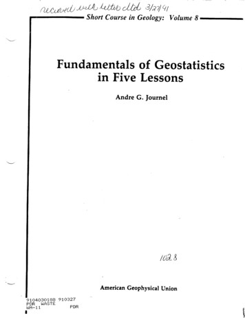
JOURNEL9(ii) Scan all data available within A to calculate theexperimental h-characteristics of spatial variability,i.e., calculate the experimental variograrn values (30).(iii) Smooth and complete the partial experimental image thus obtained into a model -y(h), available forall interdistance vectors h.(iv) Use this model y(h), or the corresponding covariance model C(h) for traditional, well-proven regression techniques, also called "kriging", see Lesson IIand III.hC(h)The most important steps, and by far the most consequential of any geostatistical study, are: step (i) - decision ofaveraging or stationarity, and, step (iii) - the modeling.Step (iv) is but well-known calculus.The decision of stationarity is implicit in all statistics,it is not particular to the geostatistical approach. Thatdecision allows defining a pool of data (area A) over whichexperimental averages and proportions will be calculatedand assumed representative of the population as a whole,not of any particular individual location (z E A).In the practice of reservoir characterization, that decision corresponds to the traditional split of the reservoirsinto zones/layers deemed homogeneous enough by the geologist. Of course, that split should not be so fine asto retain one zone per datum, for then no averaging (nostatistics) is possible.I",0h82Fig. 5. Anisotropic variogram and covarianceoa: direction of continuity02: direction across continuity&I: distance at which spatial correlation vanishes indirection al:C(Ihl,oa) 0, "y(IHL, al) sill value C(0),for all IhJ &1Let:Typical variogramsa. Z(x.),Y at IVariog
Lesson I: Statistics Review and Notations In this lesson, we will review only those basic notions of statistics that are useful to geostatistics and spatial interpolation problems. Engineering-typ