Transcription
Data Analysisusing the R Project forStatistical ComputingDaniela UshizimaNERSC Analytics/Visualization and Math GroupsLawrence Berkeley National Laboratory1
OutlineI.R-programming–––––II.Why to use RR in the scientific communityExtensibleGraphicsProfilingExploratory data analysis––RegressionClustering algorithmsIII. Case study–Accelerated laser-wakefield particlesIV. HPC–State-of-the-art2
Packages, data visualization and examplesR-PROGRAMMING3
is a language and environment forstatistical computing and graphics, aGNU project.R provides a wide variety ofstatistical (linear and nonlinearmodeling, classical statistical tests,time-series analysis, , and is highly ended adisrdebuts en.pdf4
1.Why to use R? Open-source, multiplatform, extensible; Easy on users with familiarity with S/S ,Matlab, Python or IDL; Active and growing community:– Google, Pfizer, Merck, Bank of America,Boeing, the InterContinental Hotels Group andShell.I. R-programmingII. Data AnalysisIII. Case studyIV. HPC5
2.R in the scientific community Google summer of code and projects using R-project to minelarge datasets:http://www.r-project.org/SoC08/ideas.html With Pfizer:– predict the safety of compounds, specifically carcinogenic side effectsin potential drugs.– models eliminate the expensive and time-consuming process ofstudying a large number of potential compounds in the physicallaboratory edicine-Production-Pipeline-17917-2/I. R-programmingII. Data AnalysisIII. Case studyIV. HPC6
2.1. You R with NERSC Get started with R: module load R R help() demo() help.start() source(‘your function.R’) library(package name)I. R-programmingII. Data AnalysisIII. Case studyIV. HPC7
3.Extensible Add-on packages:– Data input/output: hdf5, Rnetcdf, DICOM, etc.– Graphics: trellis, gplot, RGL, fields, etc.– Multivariate analysis: MASS, mclust, ape, etc.– Other languages: Rcpp, Rpy, R.matlab, etc.I. R-programmingII. Data AnalysisIII. Case studyIV. HPC8
4.Statistical analysis and graphs HistogramDensityBoxplotMultivariate plotConditioning plotContour plotI. R-programmingII. Data AnalysisIII. Case studyIV. HPC9
4.1.Multivariate plotsEx: Explanatory variables: solar radiation, temperature, wind and theresponse variable ozone;- use of pairs() with dataframes to check for dependencies between thevariables. data read.table('ozone.txt',header T) names(data)*1 "rad" "temp" "wind" "ozone“ pairs(data,panel.smooth)#panel.smooth locally-weighted polynomial regressionI. R-programmingII. Data AnalysisIII. Case studyIV. HPC10
4.2.Conditional plots Check the relation of the twoexplanatory variables wind,temp and the response variableozone:– Low temp: no influence of windon levels of zone;– High temp: negative relationshipbetween wind speed and ozoneconcentraton coplot(ozone wind temp,panel panel.smooth)I. R-programmingII. Data AnalysisIII. Case studyIV. HPC11
4.3. Package RGL for 3D visualization OpenGL rgl.demo.lsystem()- kernel density estimationUse Visit: https://wci.llnl.gov/codes/visit/12
Variable numberof arguments5.Profiling Where does your programspend more time?several.times - function (n, f, .) {for (i in 1:n) {f(.)}}matrix.multiplication - function (s) {A - matrix(1:(s*s), nr s, nc s)B - matrix(1:(s*s), nr s, nc s)C - A %*% B}v - NULLfor (i in 2:10) {v - ltiplication,i)) [1])}plot(v, type 'b', pch 15,main "Matrix product computation time")Also try packages:profr and proftoolsI. R-programmingII. Data AnalysisIII. Case studyIV. HPC13
Basics and beyondEXPLORATORY DATA ANALYSIS14
1. Statistical analysis Statistical modeling: check for variations in theresponse variable given explanatory variables;– Linear regression Multivariate statistics: look for structure in the data;– Clustering: Hierarchical– Dendrograms Partitioning– Kmeans (stats)– Mixture-models (mclust)I. R-programmingII. Data AnalysisIII. Case studyIV. HPC15
2.Linear regression Ex: Find the equation that best fit the data, given the decay ofradioactive emission over a 50-day period Linear regression: variables expected to be linearly related; Maximum likelihood estimates of parameters least squares;I. R-programmingII. Data AnalysisIII. Case studyIV. HPC16
2.1.Linear regressiondata read.table('sapdecay.txt',header T)attach(data)# the log(y) gives a rough idea of the decay constant, a, for these data by linear regression of log(y) against xmylm lm(log(y) x)print(mylm coefficients)# sum of squares of the difference between the observed yv and predicted yp values of y, given a specific value of parameter asumsq -function(a,xv x,yv y){yp exp(-a*xv) #predicted model for ysum((yv-yp) 2)}a seq(0.01,0.2,.005)sq sapply(a,sumsq)decayK a[min(sq) sq] #this is the least-squares estimate for the decay constantdays seq(0,50,0.1)par(mfrow c(1,3))plot(x,y,main 'Decay of radioactive emission over a 50-day period',xlab 'days')plot(a,sq,type 'l',xlab 'decay constant',ylab 'sum of squares of (observ - predicted)')matplot(decayK,min(sq),pch 19,col 'red',add T)plot(x,y); lines(days,exp(-decayK*days),col 'blue‘)detach()I. R-programmingII. Data AnalysisIII. Case studyIV. HPC17
3.Cluster analysis Hierarchical– dendrogram(stats) Partitioning– kmeans (stats)Iris dataset: 150 samples of Irisflowers described in terms of itspetal and sepal length and width Mixture-models:– Mclust (mclust)I. R-programmingII. Data AnalysisIII. Case studyIV. HPC18
3.1.Hierarchical clustering Analysis on a set ofdissimilarities, combined toagglomeration methods foranalyzing it: Dissimilarities: Euclidean,Manhattan, Methods:– ward, single, complete,average, mcquitty, medianor centroid.I. R-programmingII. Data AnalysisIII. Case studyIV. HPC19
3.2.K-means Split n observations into kclusters;– each observation belongs tothe cluster with the nearestmean.I. R-programmingII. Data Analysissetosa versicolor virginica1 048142 02363 5000III. Case studyIV. HPC20
3.3. Model-based clustering Mixture Models– Each cluster is mathematically representedby a parametric distribution;– Set of k distributions is called a mixture, andthe overall model is a finite mixture model;– Each probability distribution gives theprobability of an instance being in a givencluster.21I. R-programmingII. Data AnalysisIII. Case studyIV. HPC21
2008/apr/af-bella.htmlAccelerated laser-wakefield particlesCase study22
Knowledge discovery in LWFA sciencevia machine learning C. Geddes (LBNL) in LOASIS program headed by W.Leemans and SciDAC COMPASS project. Highlights:– Described compact electron cloudsusing minimum enclosing ellipsoids;– Developed algorithms to adaptmixture model clustering to large datasets; Science Impact:– Automated detection and analysis ofcompact electron clouds;– Derived dispersion features of electron clouds;– Extensible algorithms to other science problems;time steps Collaborators:– Tech-X– Math Group, LBNL– UCDavis, University of KaiserlauternI. R-programmingII. Data AnalysisIII. Case studyIV. HPC
Framework Goal: automate the analysis of electron bunches bydetecting compact groups of particles, with similarmomentum and spatio-temporal coherence.I. R-programmingII. Data AnalysisIII. Case studyIV. HPC24
B1. Select relevant particles Beams of interest are characterizedby high density of high-energyparticles:1. Elimination of low energy particles(px 1e10)––Representation of particle momentum in onetime step: spline interpolation onto a grid forvisualization of irregularly spaced input data.Wake oscillation: px 1e9Excludes particles of the background2. Calculation of the simulation averagenumber of particles (µs);3. Elimination of timesteps with numberof particles inferior to µs;Packages:akima, hdf5, fieldsI. R-programmingII. Data AnalysisIII. Case studyIV. HPC25
B2.Kernel-based estimation Kernel density estimators are less sensitive tothe placement of the bin edges; Goal: retrieve a dense group of particles withsimilar spatial and momentum characteristics: argmax f(x,y,px), Neighborhood: 2 µmPackages:misc3d, rgl, fieldsI. R-programmingII. Data AnalysisIII. Case studyIV. HPC26
B3. Identify beam candidates Detection of compact groups of particles independentof being a maximum in one of the variables;I. R-programmingII. Data AnalysisIII. Case studyIV. HPC27
B4. Cluster using mixture models Model and number of clusterscan be selected at run time(mclust); Partition of multidimensionalspace; Assume that the functional formof the underlying probabilitydensity follows a mixture ofnormal distributions;Packages:mclust, rglI. R-programmingII. Data AnalysisIII. Case studyIV. HPC28
B5. Evaluation of compactness Bunches of interest move at speed c, hence are nearly stationary inthe moving simulation window; Moving averages smoothes out short-term fluctuations and highlightslonger-term trends.I. R-programmingII. Data AnalysisIII. Case studyIV. HPC29
Packages, challenges and new businessesHigh performance computing30
1. Improve performance/reusability Good coding: avoid loops, vectorization; Extend R using C compiled code:– packages: Rcpp, inline Reuse your Python codes:– Package: Rpython Parallelism:– Explicit: packages Rmpi, Rpvm, nws– Implicit: packages pnmath, pnmath0 for multithreaded mathfunctions Use out-of-memory processing with– packages bigmemory and ffI. R-programmingII. Data AnalysisIII. Case studyIV. HPC31
2. What is going on HPC in R? Parallelism:– Multicore: multicore, pnmath, – Computer cluster: snow, Rmpi, rpvm, – Grid computing: GRIDR, GPU:– gputools: parallel algorithms using CUDA CULA Extremely large data:– ff: memory mapped pages of binary flat files.I. R-programmingII. Data AnalysisIII. Case studyIV. HPC
3. Nothing is perfect Limits on individual objects: on all versions ofR, the maximum number of elements of avector is 2 31 – 1; R will take all the RAM it can get (Linux only); More information, type: help(‘Memory-limits’) gc() #garbage collector object.size(your obj) #size of your objectI. R-programmingII. Data AnalysisIII. Case studyIV. HPC33
Take home Everything is an object. This means that your variables are objects, but so areoutput from analyses. Everything that can possibly be an object by some stretch ofthe imagination is an object.R works in columns, not rows. R thinks of variables first, and when you line themup as columns, then you have your dataset. Even though it seems fine in theory(we analyze variables, not rows), it becomes annoying when you have to jumpthrough hoops to pull out specific rows of data with all variables.R likes lists. If you aren’t sure how to give data to an R function, assume it will besomething like this: c(“item 1”, “item 2”) meaning “concatenate into a list the 2objects named Item 1, Item 2”. Also, “list” is different to R from “vector” and“matrix” and “dataframe” etc.Its open source. It won’t work the way you want. It has far too many commandsinstead of an optimized core set. It has multiple ways to do things, none of themreally complete. People on the mailing lists revel in their power over complexity,lack of patience, and complete inability to forgive a novice. We just have to getused to it, grit our teeth, and help them become better anding-r34
References Michael J. Crawley. Statistics: An Introduction using R. Wiley, 2005. ISBN 0470-02297-3.– data: http://www.bio.ic.ac.uk/research/mjcraw/therbook/ Robert H. Shumway and David S. Stoffer. Time Series Analysis and ItsApplications With R Examples. Springer, New York, 2006. ISBN 978-0-38729317-2 Basics– d.pdfCheat sheets– �� uts en.pdf– http://www.manning.com/kabacoff/Kabacoff MEAPCH1.pdf Intermediate– http://math.acadiau.ca/ACMMaC/Rmpi/basics.html– User-lists35
Basic but fundamentalEXTRA SLIDES36
1.Install R1.2.3.4.5.6.Download R from: http://www.r-project.orgInstall the binaryStart RPrint one of the “cheat sheets”Check the packages you may needCustomize by typing the cmd in your R session:install.packages(‘ name pkg ’)
2.Getting startedworkspace1) your question can be a valid package name or validcommand: help(graphics) or ?plot2) this will search anything that contain your query string: help.search(‘fourier’)3) which package contains the cmd? find(“plot”)4) get working directory: getwd()5) set working directory: setwd()6) variables in your R-session: ls( )7) remove your variable: rm(mytrash var)8) List the objects which contain ‘n’ ls(pat ‘n’)9) Source a function: source(‘myfunction.R’)10) Load a library library(fields)38
3. Simple syntax Basic types: numeric, character, complex or logical v1 c(7,33,1,7) #this is a vector v2 1:4#this is also a vector v3 array(1,c(4,4,3)) #create a multidimensional array i complex(real 1,imag 3) #this is a complex number Functions: n 11; print(n); sqrt(n); ifelse(n 11,n 1,n%%2)[1] 1 Operators: * / - ! %/%, , %%, sqrt(): integer division, power, modulo, square root A%*%B #matrix multiplication Packages install.packages() library(stats)39
4.Type of objects representing dataObjectModesAllow modeheterogeneity ?vectornumeric, character, complex or logical,Nofactornumeric or characterNoarraynumeric, character, complex or logicalNomatrixnumeric, character, complex or logicalNodata.framenumeric, character, complex or logicalYEStsnumeric, character, complex or logicalNolistnumeric, character, complex or logical,function, expression,YES1) Test type of object/mode: is.type()2) Coerce: as.type()Ex:x c(8,3,6,3)is.character(x)m as.character(x)Emmanuel Paradis (2009), R for Beginners40
4.1.Creating objects Arrays; Matrices; Data frame: set ofvectors of the samelength; Factor: ‘category’,‘enumerated type’ summary(.) attributes(.)41
4.2.Data input/output Graphical spreadsheet-like editor: data.edit(x) #open editor x c(5,7,2,33,9,14) x scan() data read.table(“data.txt’,header T) Ex output: write.table(d,“new file.txt”)42
5. Functions myfun function(x 1,y){ z x y z} myfun(2,3)[1] 5 Several mathematical, statistical and graphical functions; The arguments can be: “data”, formulae, expressions, . . Functions always need to be written with parentheses inorder to be executed, even if there are no parameters;– Type the function without parentheses: R will display the content ofthe function.43
5.1. Built-in functions1. Basic functions–sin(), cos(), exp(), log(), 2. Distributions–rnorm(),beta(), gamma(), binom(), cauchy(), mvrnorm(), 3. Matrix algebra–sum(), diag(), var(), det(), ginv(), eigen(), 4. Calculus–Ex: D(), integrate()5. Differential equation–Rk4() #library(odesolve)44
6.Manipulation of objects – step1 Querying data: f rep(2:4,each 3) #repeats each element of the 1st parameter 3X which(f 3) #indexes of where f 3 holds[1] 4 5 6 Related commands: seq(), unique(), sort(), rank(), order(), rev() NaN is not NA: 0/0different[1] NaN is.nan(0/0) #this is not a number[1] TRUE names c(‘mary’,’john’,NA) # use of not available45
6.1.Manipulation of objects – step2 Faster operations: apply(), lapply(), sapply(), tapply()– apply for applying functions to the rows or columns ofmatrices or dataframes apply(M,2,max) #max of col– lapply for lists lapply(list(x 1:10,y 1:30), max)– sapply for vectors sapply(m sapply(rnorm(2000),(function(x){x 2}))– tapply for tables mylist - list(c(1, 2, 2,1), c("A", "A", "B","C")) tapply(1:length(mylist), mylist)46
6.2. Create your own function Use the command line or an editor to create a function: Editor: fact - function (x){ ifelse (x 1,x*fat(x-1),1)}– Save in a file name fact.R source(‘fact.R’) fact(3) You can also save the history: savehistory(‘facthistory’) loadhistory(‘facthistory’) history(5) #see last 5 commands Tip: save filename function name47
7. Graphics Get a sense of what R can do: demo(graphics) The graphical windows are called X11 underUnix/Linux and windows under Windows Other graphical devices: pdf, ps, jpg, png x11() windows() png() pdf()48
7.1. Plot structure Graph parameter function: par(mfrow c(2, 2),las 2,cex .5,cex.axis 2.5, cex.lab 2)Changingdefaults49
7.2.Example of data plots x 1:10layout(matrix(1:3, 3, 1))par(cex 1)plot(x[2:9],col rainbow(92 2)[2:9], pch 15:(15 92 1)) #add to the plotmatplot(x,pch 17,add T);title('Using layout cmd')plot(runif(10),type 'l')plot(runif(10),type 'b')50
7.3.Creating a gif animationlibrary(fields) # for tim.colorslibrary(caTools) # for write.gifm - 400 # grid sizeC - complex(real rep(seq(-1.8,0.6, length.out m),each m), imag rep(seq(-1.2,1.2, length.out m),m))C - matrix(C, m, m)Z - 0X - array(0, c(m, m, 20))for (k in 1:20){Z - Z 2 CX[,,k] - exp(-abs(Z))}col - tim.colors(256)col[1] - "transparent"write.gif(X, “rplot-mandelbrot.gif", col col, delay 100)image(X[,,k], col col) # show final image in R51
8.Data input/output – special formats Availabity of several libraries. Ex:– Rnetcdf: netcdf functions and access to udunitscalendar conversions;– DICOM: provides functions to import andmanipulate medical imaging data via the DigitalImaging and Communications in Medicine(DICOM) Standard.– hdf5: interface to NCSA HDF5 library; read andwrite (only) the entire data52
Matlab, Python or IDL; Active and growing community: –Google, Pfizer, Merck, Bank of Americ