Transcription
January 12, 2018 15:56 1750015International Journal of Neural Systems, Vol. 28, No. 2 (2018) 1750015 (20 pages)c World Scientific Publishing Company DOI: 10.1142/S0129065717500150A Scalable Weight-Free Learning Algorithm for RegulatoryControl of Cell Activity in Spiking Neuronal NetworksInt. J. Neur. Syst. 2018.28. Downloaded from www.worldscientific.comby IOWA STATE UNIVERSITY on 06/05/18. For personal use only.Xu Zhang and Greg FoderaroMechanical Engineering andMaterials Science, Duke UniversityBox 90300 Hudson HallDurham, NC, US xz70@duke.eduCraig HenriquezBiomedical EngineeringDuke UniversityBox 90281 Hudson HallDurham, 27708, USSilvia FerrariSibley School of Mechanicaland Aerospace EngineeringCornell University, 105 Upson HallIthaca, New York, 14853, USAccepted 9 December 2016Published Online 8 March 2017Recent developments in neural stimulation and recording technologies are providing scientists with theability of recording and controlling the activity of individual neurons in vitro or in vivo, with veryhigh spatial and temporal resolution. Tools such as optogenetics, for example, are having a significantimpact in the neuroscience field by delivering optical firing control with the precision and spatiotemporal resolution required for investigating information processing and plasticity in biological brains.While a number of training algorithms have been developed to date for spiking neural network (SNN)models of biological neuronal circuits, exiting methods rely on learning rules that adjust the synapticstrengths (or weights) directly, in order to obtain the desired network-level (or functional-level) performance. As such, they are not applicable to modifying plasticity in biological neuronal circuits, in whichsynaptic strengths only change as a result of pre- and post-synaptic neuron firings or biological mechanisms beyond our control. This paper presents a weight-free training algorithm that relies solely onadjusting the spatiotemporal delivery of neuron firings in order to optimize the network performance.The proposed weight-free algorithm does not require any knowledge of the SNN model or its plasticitymechanisms. As a result, this training approach is potentially realizable in vitro or in vivo via neuralstimulation and recording technologies, such as optogenetics and multielectrode arrays, and could beutilized to control plasticity at multiple scales of biological neuronal circuits. The approach is demonstrated by training SNNs with hundreds of units to control a virtual insect navigating in an unknownenvironment.Keywords: Spiking neural networks; optogenetics; neural control; spike timing-dependent plasticity; neuromorphic; reinforcement learning.1750015-1
January 12, 2018 15:56 1750015X. Zhang et al.Int. J. Neur. Syst. 2018.28. Downloaded from www.worldscientific.comby IOWA STATE UNIVERSITY on 06/05/18. For personal use only.1.IntroductionRecent developments in neural stimulation andrecording technologies are revolutionizing the fieldof neuroscience, providing scientists with the abilityof recording and controlling the activity of individualneurons in the brain of living animals, with very highspatial and temporal resolution.1 Thanks to methods such as optogenetics, which deliver controlledcell firings to live neurons in vitro or in vivo, it isnow becoming possible to determine which regionsof the brain are primarily responsible for encoding particular stimuli and behaviors. Despite thisremarkable progress, the relationship between biophysical models of synaptic plasticity and circuitlevel learning, also known as functional plasticity,remains unknown. This important gap has beenrecently identified as one of the outstanding challenges in reverse engineering of the brain.2Many spiking neural network (SNN) learningalgorithms have been proposed to model and replicate both the synaptic plasticity and circuit-levellearning capabilities observed in biological neuronalnetworks.3–9 Experimental evidence has shown thatlearning in the brain is accompanied by changes insynaptic efficacy referred to as synaptic plasticity.10Developing learning rules for altering synaptic efficacy, commonly referred to as synaptic strength orweight, has since been the focus of both artificial neural networks (ANN) and SNN learning algorithmsto date. Along the same lines, SNN learning algorithms inspired by biological mechanisms, such asspike timing dependent plasticity (STDP),11–13 haverecently been proposed to modify synaptic weightsaccording to a learning rule model based on STDPor Hebbian plasticity, so as to optimize the networkperformance.14–19 Other SNN learning algorithmsinclude Spike-Prop20,21 and ReSuMe,22 which useclassical backpropagation and Widrow–Hoff learningrules in combination with STDP to adapt the synaptic weights so as to produce a desired SNN response.When trained by these approaches, computationalSNN have been shown to be very effective at solvingdecision and control problems in a number of applications, including delay learning, memory, and patternclassification.23–26Despite their effectiveness, none of the computational SNN learning algorithms to date havebeen implemented or validated experimentally onbiological neurons in vitro or in vivo. Suchexperimentation could help develop plausible modelslinking synaptic-level and functional-level plasticityin the brain, as well as find many potential neuroscience applications by closing the loop around therecording and the control of neuron firings. ExistingSNN learning algorithms, however, are difficult toimplement and test experimentally because they utilize learning rules for manipulating synaptic weights,while the strength of biological synapses is not easily modified in live neuronal networks. Experimentalmethods for regulating synaptic strengths in biological neurons, for example via alteration of intracellular proteins or neurotransmitters such as AMPAreceptors,27 do not lend themselves to the implementation of parallel and frequent weight changes,followed by the observation of network performance,as typically dictated by SNN learning algorithms.To overcome this fundamental hurdle, theauthors have proposed a new weight-free NN learning paradigm in which the learning rule regulates thespatiotemporal pattern of cell firings (or spike trains)to achieve a desired network-level response by indirectly modulating synaptic plasticity.28,29 Becausethis learning paradigm does not rely on manipulating synaptic strengths, in principle its learningrule can be implemented experimentally by delivering the neural stimulation patterns determined bythe algorithm to biological neurons using optogenetics or intracellular stimulation. As a first step, thisnew learning paradigm was demonstrated by showing that the synaptic strengths of a few neuronscould be accurately controlled by optimizing a radialbasis function (RBF) spike model using an analytical steepest-gradient descent method.29 As a secondstep, the method was extended to networks withup to 10 neurons by introducing an unconstrainednumerical minimization algorithm for determiningthe centers of the RBF model, such that the timings of the cell firings could be optimized.28 Thelatter approach was also shown effective at training memristor-based neuromorphic computer chipsthat aim to replicate the functionalities of biological circuitry.30,31 Because they are biologicallyinspired, these neuromorphic chips are characterizedby STDP-like mechanisms that only adjust CMOSsynaptic strengths by virtue of controllable appliedvoltages analogous to neuron firings. Therefore, theytoo are amenable to a learning paradigm that1750015-2
January 12, 2018 15:56 1750015Int. J. Neur. Syst. 2018.28. Downloaded from www.worldscientific.comby IOWA STATE UNIVERSITY on 06/05/18. For personal use only.Scalable Weight-Free Learning in Spiking Neuronal Networksseeks to regulate the spatiotemporal pattern of cellfirings (or spike trains) in lieu of the synapticstrengths.Both biological and neuromorphic circuits typically involve much larger numbers of units than havebeen previously considered by the authors. Thus, thispaper presents a new perturbative learning approachfor scaling the weight-free learning paradigm up tonetworks with hundreds of neurons. The proposedapproach is scalable because it does not rely oncomputing the spike model gradients analyticallyor numerically but rather on inferring the sign ofthe gradient by perturbation methods, effectivelyamounting to a weight-free resilient backpropagation32 algorithm for SNNs.Even in the simplest organisms, brain circuits arecharacterized by hundreds of neurons responsible forintegrating diverse stimuli and for controlling multiple functionalities.33 Because of their size, theseneuronal structures are believed to provide robustness, redundancy, and reconfigurability, characteristics that are also desirable in neuromorphic circuitsand engineering applications of computational SNNs.Recent studies on living insects have established thatmultiple forms of sensory inputs, such as visual, tactile, and olfactory information are integrated withinthe central complex (CX) circuit, to control andadapt movements to surrounding environments.33,34Inspired by these experimental studies in biology, this paper seeks to demonstrate the weightfree learning algorithm on a virtual simulation ofa walking insect in a similar arena, with multiple sensory stimuli, and sensorimotor control provided by an SNN model. The simulation results showthat when the SNN model is trained by the proposed weight-free learning algorithm, the insect iscapable to navigate new and complex terrains efficiently and robustly, based only on the inputs fromsimulated olfactory and tacticle receptors. Besidesvalidating the effectiveness of the learning algorithm, these results demonstrate that the proposedweight-free approach enables a more direct and effective transfer of biological findings to synthetic systems. Also, because the size of the SNN trainedin this paper is comparable to that of the insectCX, the weight-free algorithm could potentially berealized in vivo in living insects, to investigateand control plasticity from the synaptic level tothe functional level, via electrical or optogeneticsstimulation.2.SNN Model and ArchitectureSNNs are computational models of neuronal networks motivated by biological studies demonstrating that spike patterns are an essential component of information processing in the brain. It hasbeen hypothesized that SNNs have evolved in naturebecause they are flexible or reconfigurable, tolerantto noise or robust, require low power consumption, and can encode complex temporal and spatial inputs efficiently as correlated spike sequencesknown as spike trains.35,36 Because of these potentialadvantages, SNNs are implemented as neuromorphiccomputational platforms in software or hardware forapplications such as classification,37 computationalneuroscience,38–40 and neurorobotics.41The two crucial considerations involved in choosing the SNN model are its range of neurocomputational behaviors and its computational efficiency.42 As can be expected, the implementationefficiency typically increases with the number of features and behaviors that can be accurately reproduced,42 such that each model offers a tradeoffbetween these competing objectives. The computational neuron model that is most biophysicallyaccurate is the well-known Hodgkin–Huxley (HH)model.43 Due to its extremely low computationalefficiency, however, using the HH model to simulatelarge networks of neurons can be computationallyprohibitive.42 The simplest model of spiking neuronis the leaky integrate-and-fire (LIF). While it canonly reproduce the dynamics of a Class-1 excitableneurons that fire tonic spikes, LIF has the advantagesthat it displays the highest computational efficiencyand is amenable to mathematical analysis. Moreover, the LIF model was found to accurately reproduce the firing dynamics of CMOS neurons.44 Therefore, it is adopted in this paper to simulate all SNNarchitectures, and is reviewed in the appendix forcompleteness.Motivated by both computational NNs and biological neuronal networks for sensorimotor control,such as the insect CX,33 the following three regionsor circuits are identified in the SNN model: inputneurons (I), output neurons (O), and computational1750015-3
January 12, 2018 15:56 1750015X. Zhang et al.Output Neurons(Excitatory)ComputaƟonal Neurons(Excitatory and Inhibitory)Sensory Input Neurons(Excitatory)Sensory Input Neurons(Excitatory)Int. J. Neur. Syst. 2018.28. Downloaded from www.worldscientific.comby IOWA STATE UNIVERSITY on 06/05/18. For personal use only.Fig. 1. Computational SNN architecture where synaptic connections are illustrated for three neurons randomlyselected in each layer.or hidden neurons (H). Input neurons receive external information, such as sensory inputs, by virtue ofthe synaptic currents of structures, such as neuropils,that provide, for example, visual, olfactory, or tactileinputs. In this paper, sensory inputs are assumedto be already rate coded at the input-neuron levelin a manner proportional to the stimulus (Sec. 4).The output neurons provide the network responsewhich, in neuromorphic systems, may be decodedand used to command the actuators and, in biological systems, may consist of synaptic current inputsto motoneurons, such as for example central pattern generators (CPGs), that actuate muscles andlimbs. Neurons that are only connected to input oroutput neurons, or to each other, are referred to ashidden neurons, as illustrated in Fig. 1. Assumingthe availability of optogenetics or other firing controltool, this paper simulates a subset of input neuronsthat are light sensitive and can be made to fire oncommand.45The goal of the proposed weight-free algorithm isto determine the firing sequences to be delivered tothe input neurons (I), optically or via neural stimulation, such that the dynamic network response toall possible inputs is optimized. By stimulating thetraining neurons and/or receiving sensory inputs,the stimulus current Istim in Eq. (A.1) is modified, thereby altering the membrane potential. Whentwo or more neurons are connected by synapses, themembrane potential of the postsynaptic neuron, governed by (A.1), also depends on the synaptic currentfrom the presynaptic neurons given by,Isyn (t) gsyn (t) [Vpost (t) Esyn ],(1)where Isyn is the synaptic current from the presynaptic neurons, gsyn (t) is the synaptic conductance,Vpost is the membrane potential of the postsynaptic neuron, and Esyn is the synaptic reversal potential. Therefore, stimulating neurons in I ultimatelycauses other neurons in the SNN to fire at later times,once their membrane potentials reach Vth via synaptic current inputs.A biologically plausible model of synaptic connections is constructed by sampling uniformly andat random the distribution,46 2 D(i, j)pi,j C exp ,(2)λwhere for excitatory neurons C 0.8, and forinhibitory neurons C 0.2. The function D(i, j)represents the Euclidean distance between neuronsi and j in the neural circuit. The connection parameter λ is adjustable and, as λ approaches zero, sodoes the number of connections. The value λ 5 ischosen for all SNN models in this paper. In particular, connections are formed according to the abovedistributions within each SNN region, and pairwisebetween adjacent regions, as schematized in Fig. 1.As in many artificial and biological networks, the hidden neurons provide separation between input andoutput neurons such that, although the network isfully connected and recurrent, there are no synapticconnections between input and output neurons. Oncesynaptic connections are established probabilisticallyfrom Eq. (2), each synaptic conductance is modeledusing the alpha function,47gsyn (t) ḡsyn h(etdelay τ etrise τ),where the normalization factor is defined as, 1tt τ peak τpeakdecayriseh e e(3)(4)to ensure that the amplitude equals ḡsyn , and suchthat the conductance peaks at time: τdecayτdecay τriselntpeak .(5)(τdecay τrise )τriseImportantly, the SNN learning algorithm has nocontrol over the synaptic strengths and, thus, allsynapses change over time only by virtue of theSTDP rule (reviewed in the appendix). As observedin biological neurons,48,49 if the presynaptic neuronfires before the postsynaptic neuron, the synapseis strengthened, and if it fires after, the synapse is1750015-4
January 12, 2018 15:56 1750015Scalable Weight-Free Learning in Spiking Neuronal Networksweakened. The pair-based STDP rule can be numerically implemented in the LIF-SNN using two localvariables, xj and yi , representing low-pass filteredversions of the presynaptic spike train and the postsynaptic spike train, respectively.47 Let us considerthe synapse between neuron j and neuron i. Supposeeach spike from presynaptic neuron j contributes totrace xj at the synapse,xj dxj δ(t tfj ),(6)dtτxfInt. J. Neur. Syst. 2018.28. Downloaded from www.worldscientific.comby IOWA STATE UNIVERSITY on 06/05/18. For personal use only.tjwhere tfj denotes the firing times of the presynaptic neuron, and δ is the Dirac function. Then, thetrace xj is increased by one at tfj and subsequentlydecays with time constant τx . Similarly, each spikefrom postsynaptic neuron i contributes to a trace yiaccording to,dyiyi δ(t tfi ),(7)dtτyftiwhere tfi denotes the firing times of the postsynapticneuron. When a presynaptic spike occurs, the weightdecreases proportionally to the value of the postsynaptic trace yi , while if a postsynaptic spike occurs,a potentiation of the weight is induced.Firing rate coding is used for conversions betweenspike trains and continuous-time signals.47 Rate coding computes the mean firing frequency of a chosenset of K neurons over a time window, [t tr , t], asfollows,f (tr ) K1 zi (tr ),K i(8)where zi (tr ) denotes the number of spikes of neuroni during [t tr , t]. By this approach, the continuoustime signal or function f (tr ) can be encoded in thefiring sequences (or spike trains) of a population of Kneurons, where K can vary from one to many units.Population decoding and encoding is adopted in thispaper, because it is believed to be more robust aswell as more biologically plausible than single-unitdecoding and encoding. Also, it is routinely utilizedin biological neural systems as a useful indicator ofneural activity in sensorimotor circuits and individual cells.50,51 Finally, the SNN model described inthis section is simulated using the open-source software Neural Circuit SIMulator (CSIM),52 and theparameters provided in the appendix.3.Weight-free SNN LearningAlgorithmIn order to be applicable to biological andneuromorphic circuits, the weight-free learning algorithm presented in this section assumes that noknowledge of the SNN neuron model, connectivity,or synaptic strengths is available. It is assumed,however, that the SNN input, output, hidden, andtraining neurons, described in the previous sectioncan be stimulated or recorded from with high spatiotemporal precision. In Sec. 5, noisy sensory inputsand currents are introduced to investigate the SNNrobustness to stimulation errors by which the stimulus delivered induces multiple nearby neurons to fire.In the proposed algorithm, SNN learning andsynaptic plasticity are achieved through the application of training stimuli (e.g. optical or electricalpulses) delivered to pairs of training neurons at precise times determined via perturbative reinforcementlearning. By controlling the firing of selected trainingneurons, the algorithm indirectly modifies the synaptic strengths according to internal synaptic plasticitymechanisms, such as STDP. However, unlike existing methods,11–13 prior knowledge or models of thesemechanisms are never utilized by the weight-freelearning algorithm presented in this paper. The firing times of the training stimuli are determined solelyfrom the error between the observed SNN responseand the desired SNN response, by minimizing it inbatch mode.Whether optical or electrical, a training stimulusto an input neuron i I can be modeled as a squarepulse function, βH t ci,l 2l 1 β H t ci,l ,2si (t) wM (9)where ci,l represents the temporal center of the lthsquare pulse, M is the total number of square pulses,w is the pulse amplitude, β is the pulse duration,and H(·) is the Heaviside function. Through simulation or experimentation, the parameters of the pulsefunction are chosen such that each pulse will reliably induce neuron i to spike once and only once. Inthis case, they are chosen as w 7 10 7 (Amps)and β 0.004 (sec) based on the SNN simulation described in Sec. 2. The pulses delivered to a1750015-5
January 12, 2018 15:56 1750015Int. J. Neur. Syst. 2018.28. Downloaded from www.worldscientific.comby IOWA STATE UNIVERSITY on 06/05/18. For personal use only.X. Zhang et al.pair of neighboring neurons (i, j), where i, j I,are offset by a parameter bk that varies with thetraining epoch, indexed by k, such that the choicecj,l ci,l bk minimizes the network error over time.Let m denote the number of training cases available for which the desired SNN response to a givensensory stimulus is known. If pı (ı 1, . . . , m)denotes a vector of firing rates corresponding to aknown sensory stimulus, where each firing rate maybe defined with respect to a population (or subset)of input neurons (I), then the desired SNN responsecan be denoted by a corresponding vector u ı of firing rates that represent the desired response for oneor more subsets of output neurons (O). Then, for atraining database D {(p1 , u 1 ), . . . , (pm , u m )}, theSNN error at the kth epoch is defined as, m1 ek [uı uı (k)]T [u i ui (k)], (10)mıwhere uı (k) is the decoded SNN output at epoch k,obtained by applying Eq. (8) to the firings of the setof output neurons (O), in response to input pı .Because of the scale and the complexity of theSNN, its response to a sensory input pı needs to bedetermined experimentally. Moreover, to circumventcomputing the error gradient analytically or numerically, the sign of the error change brought aboutby the stimulus in Eq. (9) is also determined experimentally, via the following perturbation technique.Every iteration of the training algorithm, conductedover time (t), is comprised of a testing phase followed by a training phase. The testing phase consists of determining the sign of the error change overD, as brought about by training stimuli in the formof Eq. (9). The training phase consists of deliveringadditional training stimuli also in the form of Eq. (9),but such that the synaptic strengths are changed inthe direction of minimum SNN error.During the testing phase, the SNN error inEq. (10) is evaluated before and after synaptic strength perturbations. These perturbations areaccomplished by delivering the square pulses inEq. (9) with bk b0 for any k, and b0 0.002,so as to induce small perturbations in the synapticstrengths. At each epoch (k), the pair of input neurons chosen to receive a pair of training stimuli, say(i, j), i, j I, is chosen from an ordered list, N ,containing all possible neuron pairs in I, such that!, wherefrom the binomial coefficient, N 2!(NN 2)! · denotes the cardinality of a set, N N , and !denotes the factorial of a non-negative integer. Thetraining stimuli are delivered in the absence of sensory stimuli. Separately, before and after deliveringthe training stimuli, the SNN error in Eq. (10) isevaluated by delivering each (sensory stimulus) firing rate pı D to the corresponding subsets ofinput neurons (I). This is accomplished by applying pulses with the desired frequency for a durationof te 0.04, chosen such that the signal can propagate through the SNN and produce a response in theoutput neurons (O) that can be reliably decoded asoutput uı . Let ek,1 and ek,2 denote the SNN errors,computed from Eq. (10), before and after the training stimuli are delivered, respectively. Then, the signof the error change, ek ek,2 ek,1 , reflects theSNN error sensitivity to the weight perturbationsinduced by the training stimuli in Eq. (9).Based on the SNN-error sign changes during consecutive epochs, it is then possible to determinethe parameters of the square-pulse training stimuli,defined in Eq. (9), such that the SNN error is minimized over time. This is accomplished during thetraining phase, when the training stimuli in Eq. (9)are designed using the offset parameter according tothe following learning rule,bk 1 sgn( ek )b0(11)such that cj,l ci,l bk . In order to compensate forformer episodes of synaptic plasticity,53 the numberof square pulses adopted in Eq. (9) is chosen according to the following rule, 2Mk , if b0 0 and ek 0, 1Mk 1 Mk , if b0 0 and ek 0, (12) 2 Mk ,if ek 0.At each epoch (k), a new pair of neurons is selected toreceive the training signals from the ordered list N ,and the process is repeated until the error decreasesbelow a desired value or satisfies a desired stoppingcriterion.The implementation of the two phases, including the above learning rules, is summarized inthe weight-free SNN learning algorithm in Fig. 2.Figures 3 and 4 show that, without manipulatingthe synaptic weights, the training stimuli delivered1750015-6
January 12, 2018 15:56 1750015Scalable Weight-Free Learning in Spiking Neuronal Networks1Initialize SNN2Set ek,2 einit emin for k 03Set k 14while ek 1,2 emin do5Pick neurons i, j randomly6Randomly initialize b0s1 (t) si (t) and s2 (t) sj (t b0 )7 189while 2 doStimulate SNN with p1 , . . . , pm11Record and decode SNN outputs u1, . . . , um12Calculate ek, according to (10)13if 2 thenif ek,2 ek,1 then14Int. J. Neur. Syst. 2018.28. Downloaded from www.worldscientific.comby IOWA STATE UNIVERSITY on 06/05/18. For personal use only.(a)1015bk sgn(ek 1,1 ek 1,2 )b016s1 (t) si (t)s2 (t) sj (t bk )17end18(b)19end20Stimulate neurons i and j using stimuli s1 (t) and s2 (t), respectively21 1222324Fig. 4. Synaptic strength changes brought about by theweight-free algorithm’s training stimuli in Fig. 3, wherethe pair of stimuli in Fig. 3(a) potentiates the synapse asshown in (a), and the pair of stimuli in Fig. 3(b) depressesthe synapse as shown in (b).endk k 1endFig. 2. Pseudocodealgorithm.of weight-freeSNN learningmechanism. Because the weight-free algorithm doesnot control the synaptic strengths or the plasticitymechanism, it is potentially applicable to biologicalneuronal networks.4.(a)(b)Fig. 3. Training stimuli delivered by the weight-freealgorithm in Fig. 2(a), and induced action potentials oftwo pairs of pre- and post-synaptic neurons (1, 19) and(5, 22) (b), causing the weight changes in Fig. 4.by this algorithm (Fig. 3(a)) induce pre- and postsynaptic firings (Fig. 3(b)) that reliably cause synaptic strengths to change in the desired direction overtime (Fig. 4) by virtue of the underlying plasticityApplication: Virtual Insect Controland NavigationThe brains of even the simplest of organisms haveshown the remarkable ability to adapt and learn tosolve complex problems necessary for survival. Insimple organisms, such as the cockroach, physiological recordings have established that multiple formsof sensory inputs, including visual cues and tactileinformation from mechanosensors on the antenna,are integrated within the CX to control and adaptmovements to surrounding environments.34 Thesestudies utilize methods for stimulating or recordingfrom populations of brain neurons in freely behaving cockroaches using custom fabricated wire bundles inserted into the animal brain prior to releasingit into a controlled arena (Fig. 5(a)).With the recording wires in place, the animalis presented with controlled stimuli, including various obstacles, and its motion is recorded with avideo camera placed above the arena. These dataare merged so that timing of the neural activity1750015-7
January 12, 2018 15:56 1750015X. Zhang et al.Int. J. Neur. Syst. 2018.28. Downloaded from www.worldscientific.comby IOWA STATE UNIVERSITY on 06/05/18. For personal use only.relative to motion and stimuli is easily determined(Fig. 5(b)). Extracellular recording and lesion techniques link the CX to higher control of movement,and demonstrate that changes in the activity (e.g.firing rates) of individual units immediately precedechanges in the firing rates of motoneurons responsible for locomotory behaviors such as walking speed,turning, and climbing.33,54 The same wires can beused to stimulate the brain region to evoke alteredbehavior and plasticity.55Even in simple organisms, the relationshipbetween synaptic-level plasticity and higher-levellearning and behavior remains unknown. Motivatedby these experimental studies and the possibility ofGoalFig. 6. Virtual insect navigating toward the goal in acomplex terrain with hills of varying and unknown elevation (simulated in VRML56,57 ).developing plausible models of sensorimotor mechanisms and plasticity, the proposed weight-free algorithm is used to train an idealized SNN model ofinsect CX (Fig. 1) to control the motion and navigation of a virtual animal in an unknown environment.After training, the virtual insect is placed in a regionof complex topography, simulated using Matlab Virtual Reality Modeling Language (VRML),56,57 asshown in Fig. 6. Using only the sensory stimuli fromvirtual antennas, the simulated insect must navigatethe environment autonomously to reach a desiredtarget by choosing a path of minimum distance andminimum elevation, so as to minimize its energyconsumption.(a)4.1. Insect sensorimotor model(b)Fig. 5. (Color online) Track of live insect in the arenacolor coded based on the activity level of a CX unit(a). Color-coded neural (spike) activity as a functionof translational and rotational velocity over entire track(b), where warmer colors indicate higher firing frequency(taken from Ref. 55).A simple locomotion model is adopted by which thesix-legged insect moves its three rig
free learning algorithm on a virtual simulation of a walking insect in a similar arena, with multi-ple sensory stimuli, and sensorimotor control pro-vided by an SNN model. The simulation results show that when the SNN model is trained by the pro-posed weight-free learning algorithm, the i