Transcription
Fundamental Dimension Limits of AntennasEnsuring Proper Antenna Dimensions in Mobile Device DesignsRandy BancroftCenturion Wireless TechnologiesWestminster, ColoradoAbstract–The electronics industry has historically decreased the physical dimensions of theirproduct offerings. In the age of wireless products this drive to miniaturize continues. Antennas arecritical devices that enable wireless products. Unfortunately, system designers often choose antennadimensions in an ad hoc manner. Many times the choice of antenna dimensions is driven by convenience rather than through the examination of fundamental electrical limitations of an antenna. Inthis presentation the fundamental limits and the trade-offs between the physical size of an antennaand its gain, efficiency and bandwidth are examined. Finally, we examine the difficulty experiencedin determining the physical dimensions of an antenna when “non-antenna” sections of a device’sstructure may be radiating.“It was the IRE (IEEE) that embraced the new field of wireless and radio, which becamethe fertile field for electronics and later the computer age. But antennas and propagationwill always retain their identity, being immune to miniaturization or digitization.”– Harold A. WheelerElectrically Small AntennasMany customers often budget the amount of antenna volume for a given application onan ad hoc basis rather than through the use of electromagnetic analysis. Frequently thevolume is driven by customer convenience and is small enough that performance trade-offsare inherent in the antenna solution. Many times the volume allotted may be such that onlyan electrically small antenna can be used in the application.Early in a design cycle it is important to determine if the physical volume specified is,in theory, large enough electrically to allow the design of any antenna which can meet theimpedance bandwidth requirements specified. There is a fundamental theoretical limit to thebandwidth and radiation efficiency of electrically small antennas. Attempting to circumventthese theoretical limits can divert resources in an unproductive manner to tackle a problemwhich is insurmountable.
2Fundamental Dimension Limits of AntennasThe first work to address the fundamental limits of electrically small antennas was doneby Wheeler in 1947.[1] Wheeler defined an electrically small antenna as one whose maximumλ. This relation is often expressed as:dimension is less than 2πka 1(1)k 2π(radians/meter)λλ free space wavelength (meters)a radius of sphere enclosing the maximum dimension of the antenna (meters)The situation described by Wheeler is illustrated in Figure 1—1. The electrically smallantenna is in free space and may be enclosed in a sphere of radius a. ka 1.Figure 1—1 Sphere enclosing an electrically small radiating element.In 1987 the monograph Small Antennas by Fujimoto, Henderson, Hirasawa and Jamessummarized the approaches used to design electrically small antennas.[2] They also surveyedrefinements concerning the theoretical limits of electrically small antennas. It has beenestablished that for an electrically small antenna, contained within a given volume, theantenna has an inherent minimum value of Q. This places a limit on the attainable impedancebandwidth of an Electrically Small Antenna (ESA). The higher the antenna Q the smallerthe impedance bandwidth.The efficiency of an electrically small antenna is determined by the amount of lossesin the conductors, dielectrics and other materials out of which the antenna is constructedcompared with the radiation loss. This can be expressed as:ηa ηa efficiency of ESARrRr Rm(2)
Centurion Wireless TechnologiesWestminster Colorado3Rr Radiation Resistance (Ω)Rm Material Loss Resistance (Ω)The input impedance of an ESA is capacitive and in order to provide the maximumtransfer of power into the antenna’s driving point a matching network may be required. Theefficiency of the antenna and its matching network is expressed as:ηs ηa ηm(3)ηs efficiency of system (i.e. antenna and matching network)ηm efficiency of matching networkUsing common assumptions, the efficiency of the matching network is approximately:ηm ηa1 QQma(4)Qa Q of ESAQm Q of matching networkOften the efficiency of an ESA is obtained from measurement using a “Wheeler Cap.”λradius. The placementThe near field region of an ESA has been shown to reside within a 2πλradius “Wheeler Cap” on and off of an antenna produces a minimal disturbanceof a 2πof the fields. When the cap covers an antenna, the radiated and reactive power is trapped.Removing the cap allows the radiated power to propagate into free space. The dissipative lossresistance can be separated from the radiation resistance using S-parameter measurements.[3]In 1996 McLean refined and corrected earlier work on the minimum Q of an ESA.[4] Theminimum Q for an electrically small linear antenna in free space is expressed as:11 k3 a3 kaThe minimum Q for an ESA which is circularly polarized is:QL · 112Qcp 2 k3 a3 ka(5)(6)Equations (5) and (6) assume a perfect lossless matching network.In Figure 1-2 is a graph of the minimum radiation Q associated with the TE01 or TM01spherical mode for a linearly polarized antenna in free space. The exact curve was derivedby McLean and should be used in any estimates of minimum Q.The minimum Q relationship was originally derived for the case of an ESA in free space.In any practical environment an electrically small antenna is near some type of groundplaneor other structure. In 2001 Sten et al. evaluated the limits on the fundamental Q of an ESA
4Fundamental Dimension Limits of AntennasFigure 1—2 Q of an ESA vs. ka. The exact curve was derived by Mclean.[4]near a groundplane.[5] These relationships provide useful guidelines on theoretical limits tothe development of an ESA with a desired impedance bandwidth.Figure 1—3spheres.Vertical and horizontal ESA’s over a large groundplane and their enclosingThe Q for the case of a horizontal current element and a vertical current element overa groundplane are analyzed as illustrated in Figure 1—3. The formulas for the Q of both
Centurion Wireless TechnologiesWestminster Colorado5instances are found in Sten et. al.The approximate bandwidth for an RLC type circuit in terms of Q is:BW S 1 Q S(7)S S : 1 VSWRBW normalized bandwidthFigure 1—4 presents these results in a graphical form of the maximum (normalized)percent impedance bandwidth for the vertical and horizontal polarization cases with respectto the radius of a sphere which encloses the ESA. In the situation of a vertical ESA over agroundplane we find its Q is equivalent to the free space case. When a horizontal current isover a groundplane the radiation efficiency is reduced. The tangential electric field near aconductor is zero and as a horizontal ESA is brought closer and closer to the conductor surfacethe radiation decreases, the energy in the stored near fields increases, the Q becomes large,and the bandwidth becomes small. In many practical cases the proximity of a groundplanewill decrease the attainable bandwidth of an ESA.Figure 1—4
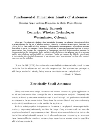
6Fundamental Dimension Limits of AntennasFigure 1—5 Dimensions of a 1.575 GHz Meanderline ESA. All dimensions are in mm.The antenna has a meanderline ESA which is matched with an electrically small section ofmicrostrip transmission line (λ/10). A 50 Ω microstrip transmission line is probe fed to acoaxial line. (x axis to right, y axis up, z axis out of page)Meander Line Antenna Impedance BandwidthWe will now use a 1.575 GHz meanderline antenna prototype to estimate the best caseimpedance bandwidth we can expect to obtain for this geometry. In Figure 1—5 the meanderline geometry is defined. The antenna consists of a meanderline element. Its inputimpedance is matched by a λ/10 section of microstrip transmission line which then feedsinto a 50 Ω feedline. The characteristic impedance of this section was determined usingcomputer optimization to provide enough series inductive reactance to cancel the large capacitive reactance of the meanderline ESA.
Centurion Wireless TechnologiesWestminster Colorado7We will assume that even though the meanderline resonator and groundplane sectionare thin, that the minimum Q restrictions for a vertically polarized ESA over an infinitegroundplane will approximately apply to this geometry.The radius of a sphere which can enclose the meanderline antenna assuming an infinitegroundplane is a 15.63 mm We calculate the free space wavelength and wavenumber whichallows us to evaluate ka.λ k 3.0 · 108c 190.48mm f1.575 · 1092π 32.987 · 10 3 radians/mmλka 32.987 · 10 3 · 15.63 0.515We can see that ka is less than one and this 1.575 GHz meanderline antenna is bydefinition an electrically small antenna. This antenna is known to be linear and polarizedvertical to the groundplane so we easily calculate the radiation Q using (5).11 9.22 3(0.515)0.515We note this value is consistent with Figure 1-2.Equation (7) provides the normalized bandwidth. We choose a 2:1 VSWR.QL 1 (0.0291) 7.66%QL 2Unfortunately this does not match with the actual percent bandwidth of 17.4%. Howcan one reconcile the measured performance verses the theoretical limit? Have we createdan antenna which violates this fundamental limit?To shed some light on this mystery let’s first determine what Q value corresponds to a17.4% (0.174) impedance bandwidth. We obtain QL 4.06 for this bandwidth. We nowneed to compute what ka value is required to produce a 4.06 value for QL . The exactsolution requires solving a cubic equation. We can estimate the value of ka from Figure 1—2.It appears ka 0.72 which is still electrically small. We know the value of k at 1.575 GHz.The value of radius is:BW a 0.72/(32.987 · 10 3 radians/ mm) 21.83mmFor the case where we have an ESA with vertical polarization over a groundplane, theradius of the antenna appears to be expanded from 15.63 mm to 21.83 mm. The explanation
8Fundamental Dimension Limits of Antennasfor this is that the radiation of the meanderline structure includes about 6.2 mm of thegroundplane. These extra currents may be seen in Figure 1—6 on the upper left and upperright vertical edges of the groundplane. Patches of current are in phase with the four verticalhigh current radiating sections on the meander line. One can see the horizontal currents onthe meander line section cancel. The complement of currents on the groundplane cancel withthe currents on the upper microstrip to form a transmission line.Figure 1—7FDTD Electric Current Magnitude Plot for the 1.575 GHz MeanderlinePrototype. The plot on the left is the current on the upper traces. The plot on the rightis of the current on the groundplane. One can see the large magnitude of the currents onthe vertical sections of the meanderline. These are essentially the only sources of radiationwhen the groundplane is enlarged.Figure 1—6 only provides the direction of electric current on the antenna. Figure 1—7is a thermal plot of the electric current magnitude normalized to the maximum current inthe modeling space. The plot on the left is of the current magnitude on the meanderlineresonator and microstrip feed line. One can see the current is concentrated at each of theshort vertical sections of the meanderline. The microstrip transmission line current is clearly
Centurion Wireless TechnologiesWestminster Colorado9Figure 1—6 FDTD Electric Current Vector Direction Plot for the 1.575 GHz MeanderlinePrototype. Red is current on upper traces. Blue is current on lower groundplane. Thecurrent on the upper sides of the groundplane contribute to the radiation sphere radiuswhich allows for a larger impedance bandwidth than when the groundplane is large.seen, as is the current along the vertical edges of the groundplane.One could be tempted to look at Figure 1—6 and conclude that the groundplane could beterminated just below the currents on each side with no negative effects. When one analyzesthe currents on this antenna with FDTD at the 2:1 VSWR band edges, and the center
10Fundamental Dimension Limits of Antennasfrequency, it may be seen that on the lower frequency limit the currents on the groundplaneedges extend almost to the end of the groundplane. The upper limit frequency doesn’tappear to drive any significant currents on the groundplane. In order to maintain the largeimpedance bandwidth we must not truncate the groundplane or it will affect the bandwidth.Figure 1—8 FDTD Electric Current Magnitude Plot for the 1.575 GHz Meanderline Prototype with 25 mm of groundplane added to each side. The upper plot is the current on theupper traces. The plot below it is of the current on the groundplane. The vertical currenton either side of the groundplane as seen in Figure 1—8 vanishes and doesn’t contribute toradiationIf one increases the width of the meanderline antenna groundplane, the impedance bandwidth will decrease until it reaches a limit. When the bandwidth limit is reached, the dimensions of the groundplane have become large enough so that the vertical currents onthe meanderline do not drive currents along the edges of the groundplane. FDTD analysisconfirms this occurs. The results are seen in Figure 1—8. One can see by comparison with
Centurion Wireless TechnologiesWestminster Colorado11Figure 1—7 no significant currents exist on the edges when the groundplane is widened. Thewidth of the electrically small matching section had to be increased to cancel the increasedcapacitive reactance of the meanderline antenna driving point as the antenna’s Q increased.When the groundplane width is increased, the bandwidth of the element decreases to5.19% bandwidth. This value is lower than our computed estimate of 7.66%. Meetingthe bandwidth limit in practice proves elusive. Recent work by Thiele et al suggests thetheoretical limit as expressed by McLean is based on a current distribution which may beunobtainable in practice.[6]Figure 1—10 shows the computed impedance bandwidth change for the baseline antennaof Figure 1-5 and after 25 mm of extra groundplane are added to each side. The reductionin impedance bandwidth is clearly illustrated.A pair of antennas were constructed using the dimensions obtained with FDTD. Figure1—11 shows the measured impedance bandwidth change for the baseline antenna and with 25mm of extra groundplane. We note the measurements correlate very well with the predictedFDTD analysis. The measured antennas had a slightly higher resonant frequency than theanalysis predicted.Meander Line Antenna Radiation PatternsThe antenna patterns computed using FDTD are essentially equivalent for the small andlarge groundplane (2.0 dB directivity). The FDTD modeling allows for “perfect” feeding ofthe antenna which minimizes any perturbation from a coaxial feedline.In practice, the gain of an electrically small antenna is bounded. This limitation hasbeen expressed by Harrington as:[7]G (ka)2 2(ka)When applied to the meanderline antenna, the maximum attainable gain for the antennaon a large groundplane (a 15.63 mm) is 1.13 dBi, when the groundplane is reduced (a 21.83 mm) we have a maximum possible gain of 2.9 dBi.Meanderline antennas were fabricated and found to match in at 1.655 GHz (4.83% from1.575 GHz). When measured, the maximum gain of the meanderline antenna with a largegroundplane is 0.3 dBi. The measured gain value of the antenna with a smaller groundplaneis 0.5 dBi. The smaller groundplane meanderline antenna generated more current along thecoaxial cable which connects the antenna to the ESA than the wider antenna. This makesmeasuring the small groundplane antenna in isolation difficult and adds loss. This measurement problem has been noted and discussed by Staub et al.[8] An electrically small antenna
12Fundamental Dimension Limits of AntennasFigure 1—9a Computed radiation patterns of the baseline (narrow groundplane) antenna(dashed lines) and the antenna with 25 mm added (solid lines) using FDTDFigure 1—9b The measured radiation patterns of the baseline (narrow groundplane) antenna (dashed lines) and the antenna with 25 mm added (solid lines)has a combination of balanced and unbalanced mode which makes pattern measurementparticularly problematic when using a coaxial (unbalanced) cable to feed the ESA.Figure 1—9a shows antenna radiation patterns predicted by FDTD analysis. The patternswith and without a large groundplane are very similar. Figure 1—9b has the measured antennaradiation patterns of the meanderline antenna with narrow and wide groundplanes. The YZplane cut is directly through the connecting cable. One can see the electrically smallestantenna is most perturbed by the cable connection. The other two planes have patterns foreach of the two antennas which are very similar.
Centurion Wireless TechnologiesWestminster Colorado13Figure 1—10 S11 dB of the baseline (narrow) antenna and the antenna with 25 mm addedto each side as predicted with FDTDConclusionIn a number of applications such as wireless PCMCIA cards, ESA’s have been implemented that have adequate impedance bandwidth, and are well matched. Later a groundplane change considered to be minor would be implemented by a customer on a board turnand the antenna would no longer be matched. In some cases after matching the impedancebandwidth would decrease or in some cases increase. Fundamental limitations on antennasize versus impedance bandwidth brings order to what can appear to be mysterious changesin antenna performance.When possible, an electrically large antenna should be implemented. This allows forthe possibility of a large impedance bandwidth. A large impedance bandwidth often allowsthe electrically large antenna to continue functioning even when loaded by objects in itsenvironment. Electrically large antennas generally have higher efficiencies than ESAs. Whena design doesn’t allow for a full size antenna, it is imperative to understand the trade-offsinvolved when using an ESA to realize a successful design.
14Fundamental Dimension Limits of AntennasFigure 1—11 S11 dB of the baseline (narrow) antenna and the antenna with 25 mm addedto each side (measured)References:[1] H.A. Wheeler,“Fundamental Limits of Small Antennas,” Proceedings of The I.R.E. (IEEE), December 1947, pg.1479-1484[2] K. Fujimoto, A. Henderson, K. Hirasawa and J.R. James, Small Antennas, John Wiley & Sons Inc. 1987[3] H.A. Wheeler,“The Radiansphere Around a Small Antenna,” Proceedings of The I.R.E. (IEEE), August 1959,Vol. 47[4] James S. McLean, “A Re-Examination of the Fundamental Limits on The Radiation Q of Electrically SmallAntennas,” IEEE Transactions on Antennas and Propagation Vol 44, NO. 5, May 1996, pg. 672-675[5] Johan C.—E. Sten, Arto Hujanen, and Päivi K. Koivisto, “Quality Factor of an Electrically Small AntennaRadiating Close to a Conducting Plane,” IEEE Transactions on Antennas and Propagation, VOL. 49, NO. 5May 2001, pp. 829—837[6] Gary A. Thiele, Phil L. Detweiler, and Robert P. Penno, “On the Lower Bound of the Radiation Q for ElectricallySmall Antennas,” IEEE Transactions on Antennas and Propagation, VOL. 51, NO. 6 June 2003, pp. 1263—1268[7] Roger F. Harrington, “Effect of Antenna Size on Gain, Bandwidth, and Efficiency,” Journal of Research of theNational Bureau of Standards—D, Radio Propagation VOL. 64D, No. 1, January-February 1960, pp. 1—12[8] O. Staub, J.F. Zürcher, and A. Skrivervlk, “Some Considerations on the Correct Measurement of the Gainand Bandwidth of Electrically Small Antennas,” Microwave and Optical Technology Letters, VOL. 17, NO. 3February 20, 1998, pp. 156—160
dimensions in an ad hoc manner. Many times the choice of antenna dimensions is driven by conve-nience rather than through the examination of fundamental electrical limitations of an antenna. In this presentation the fundamental limits and the trade-offs between the physical size of an antenna and its