Transcription
AppendixCFinite Element AnalysisUsing ANSYSC.1 INTRODUCTIONANSYS is the original (and commonly used) name for ANSYS Mechanical or ANSYSMultiphysics, general-purpose finite element analysis software. ANSYS, Inc actuallydevelops a complete range of CAE products, but is perhaps best known for ANSYS Mechanical & ANSYS Multiphysics. The academic versions of these commercial productsare referred to as ANSYS Academic Research, ANSYS Academic Teaching Advanced,Introductory etc. All of these products are general purpose finite element self containedanalysis tools incorporating preprocessing (geometry creation, meshing), solver and postprocessing modules in a unified graphical user interface (GUI). For the remainder of thisappendix, when we state ‘‘ANSYS’’, we mean the FEA capability of either the commercial or academic ANSYS Inc. products discussed above. Further we are limiting our discussion to the traditional (or ‘‘classic’’) user interface of ANSYS, not the ANSYSWorkbench environment.One of the advantages of ‘‘ANSYS’’ is the user-programmable capability. TheANSYS Command Language contains several thousand commands relating to creatinggeometry, mesh, boundary conditions, solver settings & many other features. A subsetof these commands are termed ANSYS Parametric Design Language (APDL), and focus on managing parameters, macros, if-then-else branching, do-loops, and scalar, vector and matrix operations. For example, if multiple analyses are required with differentvalues of parameters, do-loops can be used to change parameters, or the Optimizationmodule (/OPT) can be used to automatically manage parameters & populate a responsesurface.There are two different modes of performing finite element analysis in ANSYS:batch and interactive modes. The batch mode requires an input file of commands andexecutes it from the command line, while the interactive mode turns on the graphical userinterface and shows the result of each user action (picked from a menu or typed as acommand) in a graphics window. The batch mode is best suited for those experiencedwith the ANSYS Command Language. In this tutorial, only the interactive mode will beexplained.There are two different modes of inputting commands in ANSYS: graphic mode andtext mode. In the graphic mode, the user can pick commands and type in required datavalues. Thus, there is no need to memorize all commands. This mode is beneficial in asense that the user can see the result of each command in the graphic window. In the textmode, the user type in commands and data in the command area. In this case, the usershould remember what command should be used to perform a particular action. However,the text mode has its own advantages. For example, during the design process, the user363
364Appendix CFinite Element Analysis Using ANSYSmay want to perform the analysis multiple times with different values of parameters. Insuch a case, the user can prepare a text file of all commands and then input the file as aninput command file. In fact, all actions in the graphic mode are stored as commands in atext file, jobname.log. Thus, it would be a good practice to prepare the initial model usingthe graphic mode, and then, modify the input file for the further modification. In thischapter, we will present two tutorials using the graphic mode, and then will present several examples in Chapters 2–7 using the text mode.C.2 GETTING STARTANSYS can be started in different ways. In this tutorial, we will start ANSYS in thetraditional mode. To access ANSYS program on Windows systems, choose Start Programs ANSYS 11.0 ANSYS. This command will open ANSYS window asshown in Figure C.1. The ANSYS window is composed of different areas. The graphicarea shows geometries and finite elements as well as results of simulation. The mainmenu contains primary ANSYS functions. The user can directly type in commands inthe command area. The standard toolbox collects commands that are frequently used.The utility menu contains utility functions that are available throughout the ANSYSsession.In order to finish ANSYS, choose File Exit command. Then, Exit from ANSYSwindow will show up as shown in the right-lower corner of Figure C.1. Choose a properoption and OK to finish the program.ANSYS has its full documents in help menu. In the utility menu, choose Help HelpTopics. Then ANSYS 11.0 Documentation windows will show up. In this documentation,the user can find all manuals and tutorials available in ANSYS.Figure C.1 Layout of ANSYS main window and exit window
C.3Static Analysis of a Corner Bracket365C.3 STATIC ANALYSIS OF A CORNER BRACKET2A. Problem DescriptionThis is a simple, single load step, structural static analysis of the corner angle bracketshown in Figure C.2. The upper left-hand pin hole is constrained (welded) around itsentire circumference, and a tapered pressure load is applied to the bottom of the lowerright-hand pin hole. The objective of the problem is to demonstrate the typical ANSYSanalysis procedure. The US Customary system of units is used.The dimensions of the corner bracket are shown in the figure. The bracket is made ofA36 steel with a Young’s modulus of 30E6 psi and Poisson’s ratio of 0.27. Since thebracket is thin in the z-direction (1/2 inch thick) compared to its x and y dimensions, andsince the pressure load acts only in the x-y plane, the problem can be assumed as planestress. We will use solid modeling to generate the two-dimensional model and automatically mesh it with nodes and elements. (Another alternative in ANSYS is to create thenodes and elements directly.)If your system includes a Flash player (Macromedia, Inc.), one can view demonstration videos of each step by pointing the web browser to the following URL address: http://www.ansys.com/techmedia/structural tutorial videos.htmlB. Building the GeometryIn order to perform the finite element analysis, we need to create the geometry, and elements, and to apply boundary conditions. This step is called pre-processing.Step 1: Define rectanglesThere are several ways to create the model geometry within ANSYS, some moreconvenient than others. The first step is to recognize that you can construct the bracketeasily with combinations of rectangle and circle primitives. Decide where the origin willbe located and then define the rectangle and circle primitives relative to that origin. Thelocation of the origin is arbitrary. Here, use the center of the upper left-hand hole. ANSYSdoes not need to know where the origin is. Simply begin by defining a rectangle relativeto that location. In ANSYS, this origin is called the global origin.Figure C.2 Corner bracket stress analysis problem2By the courtesy of ANSYS, Inc.
366Appendix CFinite Element Analysis Using ANSYS1. Choose Main Menu Preprocessor Modeling Create Areas Rectangle By Dimensions2. Enter the following data to create the first rectangle: X1 ¼ 0; X2 ¼ 6; Y1 ¼ 1; Y2 ¼ 1 (Note: Press the Tab key between entries)3. Apply to create the first rectangle.4. Enter the following data to create the second rectangle: X1 ¼ 4; X2 ¼ 6; Y1 ¼ 1; Y2 ¼ 35. OK to create the second rectangle and close the dialog box.Now the geometry should look like the figure below.Step 2: Change plot controls and replotThe area plot shows both rectangles,which are areas, in the same color. To moreclearly distinguish between areas, turn on areanumbers and colors. The ‘‘Plot NumberingControls’’ dialog box on the Utility Menu controls how items are displayed in the GraphicsWindow. By default, a ‘‘replot’’ is automatically performed upon execution of the dialogbox. The replot operation will repeat the lastplotting operation that occurred (in this case,an area plot).1. Choose Utility Menu Plot Ctrls Numbering2. Turn on area numbers.3. Choose OK to change controls, close the dialog box, and replot.
C.3Static Analysis of a Corner Bracket367Before going to the next step, save the work you have done so far.ANSYS stores any input data in memory to the ANSYS database.To save that database to a file, use the SAVE operation, availableas a tool on the Toolbar. ANSYS names the database file using theformat jobname.db. You can check the current jobname at any timeby choosing Utility Menu List Status Global Status. You canalso save the database at specific milestone points in the analysis(such as after the model is complete, or after the model is meshed)by choosing Utility Menu File Save As and specifying differentjobnames (model.db, or mesh.db, etc.).It is important to do an occasional save so that if you make amistake, you can restore the model from the last saved state. Yourestore the model using the RESUME operation, also available onthe Toolbar. (You can also find SAVE and RESUME on the UtilityMenu, under File.)Step 3: Change working plane to polar and create first circleThe next step in the model construction is to create the half circle ateach end of the bracket. You will actually create a full circle on eachend and then combine the circles and rectangles. To create the circles,you will use and display the working plane. You could have shown theworking plane as you created the rectangles but it was not necessary.Before you begin however, first ‘‘zoom out’’ within the Graphics Window so you cansee more of the circles as you create them. You do this using the ‘‘Pan-Zoom-Rotate’’dialog box, a convenient graphics control box you’ll use often in any ANSYS session.Choose Utility Menu PlotCtrls Pan, Zoom, RotateClick on small dot once to zoom out.Close dialog box.Choose Utility Menu WorkPlane Display Working Plane (toggle on)Notice the working plane origin is immediately plotted in theGraphics Window. It is indicated by the WX and WY symbols;right now coincident with the global origin X and Y symbols.Next you will change the WP type to polar, change the snap increment, and display the grid.5. Choose Utility Menu WorkPlane WP Settings6. Click on Polar.7. Click on Grid and Triad.8. Enter .1 for snap increment.9. OK to define settings and close the dialog box.1.2.3.4.
368Appendix CFinite Element Analysis Using ANSYS10. Choose Main Menu Preprocessor Modeling Create Areas Circle Solid CircleBe sure to read prompt before picking.11. Pick center point at: WP X ¼ 0; WP Y ¼ 0; Radius ¼ 1 (in Graphics Windowshown below)12. Choose OK to close picking menu.13. Toolbar: SAVE DB.Step 4: Move working plane and create second circleTo create the circle at the other end of the bracket inthe same manner, you need to first move the workingplane to the origin of the circle. The simplest way to do this without entering number offsets is to move the WP to an average keypoint location by picking the keypoints at thebottom corners of the lower, right rectangle.1. Choose Utility Menu WorkPlane Offset WP to Keypoints2. Pick keypoint at lower left corner of rectangle.3. Pick keypoint at lower right of rectangle.4. OK to close picking menu.5. Choose Main Menu Preprocessor Modeling Create Areas Circle Solid Circle6. Pick center point at: WP X ¼ 0; WP Y ¼ 0; Radius ¼ 17. OK to close picking menu.8. Toolbar: SAVE DB.
C.3Static Analysis of a Corner Bracket369Step 5: Add areas.Now that the appropriate pieces of the model are defined (rectangles and circles), youneed to add them together so the model becomes one continuous piece. You do this withthe Boolean add operation for areas.1. Choose Main Menu Preprocessor Modeling Operate Booleans Add Areas2. Choose Pick All for all areas to be added.3. Toolbar: SAVE DB.Step 6: Create line fillet.1. Choose Utility Menu PlotCtrls Numbering2. Turn on line numbering.3. OK to change controls, close the dialog box, and automatically replot.
370Appendix CFinite Element Analysis Using ANSYS4. Choose Utility Menu WorkPlane DisplayWorking Plane (toggleoff)5. Choose Main Menu Preprocessor Modeling Create Lines Line Fillet6. Pick lines 17 and 8.7. OK to finish picking lines (in picking menu).8. Enter 0.4 as the radius.9. OK to create line fillet and close the dialogbox.10. Choose Utility Menu Plot LinesStep 7:Create fillet area.1. Choose Utility Menu PlotCtrls Pan,Zoom, Rotate2. Click on Zoom button.3. Move mouse to fillet region, click left button,move mouse out and click again.4. Choose Main Menu Preprocessor Modeling Create Areas Arbitrary ByLines5.6.7.8.9.Pick lines 4, 5, and 1.OK to create area and close the picking menu.Click on Fit button in Pan, Zoom, Rotate dialog box.Close the Pan, Zoom, Rotate dialog box.Choose Utility Menu Plot Areas
C.3Static Analysis of a Corner Bracket37110. Toolbar: SAVE DB.Step 8:Add areas together.1. Choose Main Menu Preprocessor Modeling Operate Booleans Add Areas2. Pick All for all areas to be added.3. Toolbar: SAVE DB.Step 9:Create first pin hole.1. Choose Utility Menu WorkPlane Display Working Plane (toggle on)2. Choose Main Menu Preprocessor Modeling Create Areas Circle Solid Circle3. Pick center point at: WP X ¼ 0; WP Y ¼ 0; Radius ¼0:44. OK to close picking menu.Step 10:Move working plane and create second pin hole.1. Choose Utility Menu WorkPlane Offset WP to Global Origin2. Choose Main Menu Preprocessor Modeling Create Areas Circle Solid Circle3. Pick center point at: WP X ¼ 0; WP Y ¼ 0; Radius ¼ 0:4 (in Graphics Window)4. OK to close picking menu.5. Utility Menu WorkPlane DisplayWorking Plane (toggle off)6. Utility Menu Plot LinesIf you plot areas, it appears that one of thepin hole areas is not there. However, it isthere (as indicated by the presence of itslines), you just can’t see it in the final display of the screen. That is because thebracket area is drawn on top of it. An easyway to see all areas is to plot the linesinstead.7. Toolbar: SAVE DB.Step 11:Subtract pin holes from bracket.1. Choose Main Menu Preprocessor Modeling Operate Booleans Subtract Areas2. Pick bracket as base area from which to subtract.
372Appendix CFinite Element Analysis Using ANSYS3. Apply (in picking menu).4. Pick both pin holes as areas to besubtracted.5. OK to subtract holes and close pickingmenu.Step 12: Save the database as model.db.At this point, you will save the database toa named file—a name that represents the modelbefore meshing. If you decide to go back andremesh, you’ll need to resume this database file.You will save it as model.db.1. Choose Utility Menu File SaveAs2. Enter model.db for the database filename.3. OK to save and close dialog box.C. Define MaterialsStep 13:Set preferences.In preparation for defining materials, you will set preferences so that only materialsthat pertain to a structural analysis are available for you to choose.To set preferences:1. Choose Main Menu Preferences2. Turn on structural filtering. The options may differ from what is shown here sincethey depend on the ANSYS product you are using.3. OK to apply filtering and close the dialog box.Step 14: Define material properties.To define material properties for this analysis, there is only one material for the bracket,A36 Steel, with given values for Young’s modulus of elasticity and Poisson’s ratio.
C.31.2.3.4.5.Static Analysis of a Corner Bracket373Choose Main Menu Preprocessor Material Props Material ModelsDouble-click on Structural, Linear, Elastic, Isotropic.Enter 30e6 for EX and 0.27 for PRXY.OK to define material property set and close the dialog box.In the Define Material Model window, choose Material ExitStep 15: Define element types and options.In any analysis, you need to select from a library of element types and define theappropriate ones for your analysis. For this analysis, you will use only one element type,PLANE82, which is a 2-D, quadratic, structural, higher-order element. The choice of a
374Appendix CFinite Element Analysis Using ANSYShigher-order element here allows you to have a coarser mesh than with lower-order elements while still maintaining solution accuracy. Also, ANSYS will generate some triangle shaped elements in the mesh that would otherwise be inaccurate if you used lowerorder elements (PLANE42). You will need to specify plane stress with thickness as anoption for PLANE82. (You will define the thickness as a real constant in the next step.)1.2.3.4.5.6.7.8.9.Choose Main Menu Preprocessor Element Type Add/Edit/DeleteChoose Add. . . button in Element Types window.In Library of Element Types window, Choose Solid.Choose 8node 82, which is the 8-node quad element type (PLANE82).OK to apply the element type and close the dialog box.Choose Options. . . button in Element Types window.Choose plane stress with thickness option for element behavior.OK to specify options and close the options dialog box.Close the element type dialog box.
C.3Static Analysis of a Corner Bracket375Step 16: Define real constants.For this analysis, since the assumption is plane stresswith thickness, you will enter the thickness as a real constant for PLANE82. To find out more information aboutPLANE82, you will use the ANSYS Help System in thisstep by clicking on a Help button from within a dialog box.1. Choose Main Menu Preprocessor Real Constants Add/Edit/Delete2. Choose Add. . . button for a real constant set.3. OK for PLANE82.4. Help to get help on PLANE82.5. Hold left mouse button down to scroll through element description.6. Close the Help window7. Enter .5 for THK.8. OK to define the real constant and close the dialog box.9. Close the real constant dialog box.D. Generate MeshStep 17:Mesh the area.One nice feature of the ANSYS program is that you can automatically mesh the model without specifying any mesh size controls. This is using what is called a default mesh.If you’re not sure how to determine the mesh density, let ANSYS try it first! Meshing thismodel with a default mesh, however, generates more elements than are allowed in the
376Appendix CFinite Element Analysis Using ANSYSANSYS ED program. Instead you will specify a global element sizeto control overall mesh density.Choose Main Menu Preprocessor Meshing Mesh ToolSet Global Size control.Type in 0.5.OK.Choose Area Meshing.Click on Mesh.Pick All for the area to be meshed (in picking menu). Closeany warning messages that appear.8. Close the Mesh Tool.1.2.3.4.5.6.7.The mesh you see on your screen may vary slightly from the mesh shown here. As aresult of this, you may see slightly different results during postprocessing.Step 18: Save the database as mesh.db.Here again, you will save the databaseto a named file, this time mesh.db.1. Choose Utility Menu File Save as2. Enter mesh.db for database filename.3. OK to save file and close dialog box.E. Apply LoadsNow, we finish preprocessing phase and move on to the solution phase. A new, staticanalysis is the default, so you will not need to specify analysis type for this problem. Also,there are no analysis options for this problem.Step 19: Apply displacement constraints.You can apply displacement constraints directly to lines.1. Choose Main Menu Solution Define Loads Apply Structural Displacement On Lines
C.3Static Analysis of a Corner Bracket3772. Pick the four lines around left-hand hole(Line numbers 10, 9, 11, 12).3. OK (in picking menu).4. Click on All DOF.5. Enter 0 for zero displacement.6. OK to apply constraints and close dialogbox.7. Choose Utility Menu Plot Lines8. Toolbar: SAVE DB.Step 20: Apply pressure load.Now apply the tapered pressure load to the bottom, right-hand pin hole. (‘‘Tapered’’here means varying linearly.) Note that when a circle is created in ANSYS, four linesdefine the perimeter. Therefore, apply the pressure to two lines making up the lower halfof the circle. Since the pressure tapers from a maximum value (500 psi) at the bottom ofthe circle to a minimum value (50 psi) at the sides, apply pressure in two separate steps,with reverse tapering values for each line. The ANSYS convention for pressure loading isthat a positive load value represents pressure into the surface (compressive).1. Choose Main Menu Solution Define Loads Apply Structural Pressure On Lines2. Pick line defining bottom left part of the circle (line 6).3. Apply.4. Enter 50 for VALUE.
378Appendix CFinite Element Analysis Using ANSYS5. Enter 500 for optional value.6. Apply.7. Pick line defining bottom right partof circle (line 7).8. Apply.9. Enter 500 for VALUE.10. Enter 50 for optional value.11. OK.12. Toolbar: SAVE DB.F. Obtain SolutionStep 21:Solve.1. Choose Main Menu Solution Solve Current LS2. Review the information in the status window, then choose File Close (Windows), or Close (X11/Motif), to close the window.3. OK to begin the solution. Choose Yes to any Verify messages that appear.4. Close the information window when solution is done.ANSYS stores the results of this one load step problem in the database and in theresults file, Jobname.RST (or Jobname.RTH for thermal, Jobname.RMG for magnetic, and Jobname.RFL for fluid analyses). The database can actually contain only oneset of results at any given time, so in a multiple load step or multiple substep analysis,ANSYS stores only the final solution in the database. ANSYS stores all solutions inthe results file.
C.3Static Analysis of a Corner Bracket379G. Review ResultsNow, we finish the solution phase and move to the postprocessing phase. The results yousee may vary slightly from what is shown here due to variations in the mesh.Step 22:Enter the general postprocessor and read in the results.1. Choose Main Menu General Postproc Read Results First SetStep 23: Plot the deformed shape.1. Choose Main Menu General Postproc Plot Results Deformed Shape2. Choose Def undeformed.3. OK. You can also produce an animatedversion of the deformed shape:4. Choose Utility Menu Plot Ctrls Animate Deformed Shape5. Choose Def undeformed.6. OK to start animation.7. Make choices in the Animation Controller, if necessary, then choose Close.Step 24:Plot the von Mises equivalent stress.1. Choose Main Menu General Postproc Plot Results Contour Plot NodalSolu2. Choose Stress item to be contoured.3. Scroll down and choose von Mises stress.4. OK.The colors in the contour plot stand for the level of von Mises stress. The maximum stress occurs at the fixed pin hole. The value of stress can be read from thecolor legend in the bottom of the graphic screen. Note that the color legend can beshown on the right side of graphic screen. You can also produce an animated version of these results:5. Choose Utility Menu Plot Ctrls Animate Deformed Results
380Appendix C6.7.8.9.Choose Stress item to be contoured.Scroll down and choose von Mises SEQV.OK.Make choices in the Animation Controller, if necessary, then choose Close.Step 25:1.2.3.4.Finite Element Analysis Using ANSYSList reaction solution.Choose Main Menu General Postproc List Results Reaction SoluOK to list all items and close the dialog box.Scroll down and find the total vertical force, FY.Choose File Close (Windows), or Close (X11/Motif), to close the window.
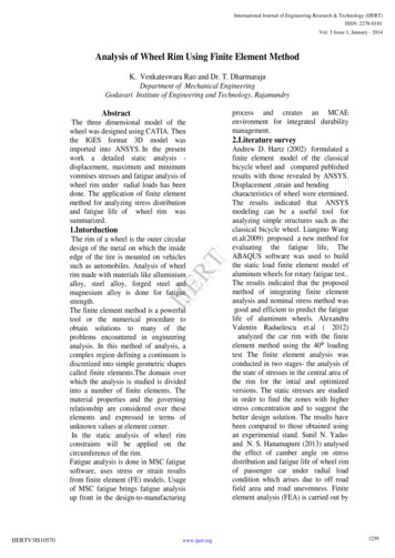
C.4Examples in the Text381The value of 134.61 is comparable to the total pin load force. Note that the valuesshown are representative and may vary from the values you obtain. There are many otheroptions available for reviewing results in the general postprocessor. You have finished theanalysis. Exit the program in the next step.Step 26: Exit the ANSYS program.When exiting the ANSYS program, you can save the geometry and loads portions ofthe database (default), save geometry, loads, and solution data (one set of results only),save geometry, loads, solution data, and postprocessing data (i.e., save everything), orsave nothing. You can save nothing here, but you should be sure to use one of the othersave options if you want to keep the ANSYS data files.1. Toolbar: Quit.2. Choose Quit - No Save!3. OK.C.4 EXAMPLES IN THE TEXTThe tutorial in the previous section was performed using graphical user interface(GUI) in which the user chooses commands using the menu. Then the GUI interpretsthese inputs into commands and sends them to ANSYS program. However, it is possible to type in ANSYS commands directly in the Command area. You can preparecommands in text editor and copy and paste them to the Command area. Or, you cansave commands as a file and read them using Utility Menu File Read InputFrom. . . In this section, we present various example problems in the text using thecommand mode.Example 2.4 – Two–bar Truss StructureThe two–bar truss shown in Figure C.3 has circular cross-sections with diameter of0.25cm and Young’s modulus E ¼ 30 106 N cm2 . An external force F ¼ 50 N is applied in the horizontal direction at Node 2. Calculate the displacement of each node andstress in each element. The commands that can perform the finite element analysis islisted in Table C.1.The detailed explanation of each command can be found by typing HELP, COMMAND in the command area. In ANSYS command lines, any text after ‘‘!’’ is consideredas a comment; i.e., ignored by the program. The above commands are composed of threephases: preprocessing (/PREP7), solution (/SOLUTION), and postprocessing (/POST1).Each phase is ended using FINISH command. In this simple example, we generate nodesFigure C.3 Two–bar truss
382Appendix CFinite Element Analysis Using ANSYSTable C.1 ANSYS Commands for Two–bar Truss DISP,1PRDISPPRESOL,ELEMFINISH!!!!Start preprocessingElement type 1 2D Truss elementElastic modulus of material set 1Cross-sectional area ofreal constant set 1! Define Node 1 (0, 0)! Define Node 2 (12, 8)! Define Node 3 (12, 0)!!!!!Use Element type 1Use material set 1Use real constant set 1Create Element 1 (N1 - N2)Create Element 2 (N2 - N3)!!!!Fix all DOFs of Node 1Fix all DOFs of Node 3Apply Fx 50N at Node 2Finish preprocessing! Start simulation! Solve the matrix equation! Finish simulation!!!!!!Start postprocessingChoose the first result setPlot the deformed geometryPrint out the nodal displacementPrint out all element resultsFinish postprocessingand elements directly (N and E commands). Displacement boundary conditions are imposed using D command, and the nodal force is applied using F command. The outputfrom the PRDISP command is shown 8108E-030.000Note that the nodal displacements are the same with Example 2.4 in Chapter 2. Theoutput from PRESOL command is shown below:EL 1MFORX SAXL NODES 160.0931224.2EL 2MFORX SAXL NODES 2-33.333-679.062MAT 1LINK1EPELAXL 0.0000413MAT 1EPELAXL -0.000023LINK1
C.4Examples in the Text383MFORX, SAXL, and EPELAXL are, respectively, element force, axial stress, and axialstrain. Note that Element 1 is in tension, while Element 2 is in compression. The outputfrom PLDISP command is shown below:In general, the displacements are relatively small. Thus, most graphical postprocessors amplify the displacement so that the deformed shape of the truss can be shown in thefigure.Example 2.5 – Plane Truss with Three ElementsThe plane truss shown in Figure C.4 consists of three members connected to each otherand to the walls by pin joints. The members make equal angles with each other and element 2 is vertical. The members are identical to each other with properties: Young’s modulus E ¼ 206 109 Pa, cross-sectional area A ¼ 1 10 4 m2 , and length L ¼ 1 m. Aninclined force F ¼ 20; 000 N is applied at node 1. Solve for the displacements at node 1and stresses in the three elements.One of powerful capabilities in ANSYS is parametric programming. The user canassign a value to a variable and use it as an argument in the following commands. Forexample, we define a variable val ¼ 1 sqrtð2Þ, and then, use it in the definition ofFigure C.4 Plane structure with three truss elements
384Appendix CFinite Element Analysis Using ANSYSTable C.2 ANSYS Commands for Three Truss Elements ng L,ELEMFINISH!!!!Start preprocessingElement type 1 2D Truss elementElastic modulus of material set 1Cross-sectional area ofreal constant set 1! Define nodal coordinates!!!!!!Use Element type 1Use material set 1Use real constant set 1Create Element 1Create Element 2Create Element 3!!!!!!Fix all DOFs of Node 2Fix all DOFs of Node 3Fix all DOFs of Node 4Apply force at Node 2Apply force at Node 2Finish preprocessing! Start simulation! Solve the matrix equation! Finish simulation!!!!!!Start postprocessingChoose the first result setPlot the deformed truss geometryPrint out the nodal displacementPrint out all element resultsFinish postprocessingnodal coordinates, as N,3,val, val. The variable can be an array or matrix.Table C.2 shows the list of ANSYS commands for plane truss. The output from thePRDISP command is shown 5767E-030.00000.00000.0000Note that the nodal displacements are the same as in Example 2.5 in Chapter 2. Theoutput from PRESOL command is shown below:
C.4EL 1 NODES 1MFORX -3450.9SAXL -0.34509E 08Examples in the Text3 MAT 3851EPELAXL -0.000168EL 2 NODES 12 MAT MFORX -9428.1SAXL -0.94281E 08 EPELAXL -0.0004581EL 3 NODES 14 MAT MFORX 12879.SAXL 0.12879E 09 EPELAXL 0.0006251The output from PLDISP command is shown in Figure C.5.Example 2.6 – Space Truss ProblemUse the finite element method to determine the displacements and forces in the spacetruss, shown in Figure C.6. The coordinates of the nodes in meter units are given in theFigure C.5 Deformed shape of the plane structure with three truss elementsFigure C.6 Three–bar space truss structure
386Appendix CFinite Element Analysis Using ANSYStable. Assume Young’s modulus E ¼
Using ANSYS C.1 INTRODUCTION ANSYS is the original (and commonly used) name for ANSYS Mechanical or ANSYS Multiphysics, general-purpose finite element analysis software. ANSYS, Inc actually develops a complete range of CAE products, but is perhaps best known for ANSYS Me-chanical & ANSYS Mu