Transcription
Univerza v LjubljaniFakulteta za matematiko in fizikoOddelek za fizikoSmer: naravoslovna fizikaBARCHAN DUNESSeminar 2Author: Barbara HorvatMentor: prof.dr.Rudolf Podgornik
AbstractSand dunes occur throughout the world, from coastal and lakeshore plains to arid desert regions. Not juston Earth but also on Mars, Venus etc. In this seminar I am going to talk about barchan dunes: about theircreation, movement and shape.
1DunesDef. A sand dune is a hill made by the wind on the coast or in a desert or by the water under the water.With regard to the wind direction we know two types of dunes: longitudinal dunes also called Seif dunes, elongate parallel to the prevailing wind, possibly caused bya larger dune having its smaller sides blown away. They are sharp-crested and range up to 300m inheight and 300km in length. transverse dunes which are horizontal to the prevailing wind, probably caused by a steady buildup ofsand on an already existing minuscule mound. They appear in regions of mainly unidirectional windand high sand availability.On the other hand we know also different shapes that were made under different wind conditions so to speakunder different wind directions: Crescenticthe most common dune form on Earth (and on Mars) is the crescentic. Crescent-shaped moundsgenerally are wider than long. The slipface is on the dune’s concave side. These dunes form underwinds that blow from one direction, and they also are known as barchans, or transverse dunes. Sometypes of crescentic dunes move faster over desert surfaces than any other type of dune. Linearstraight or slightly sinuous sand ridges typically much longer than they are wide are known as lineardunes. They may be more than 160km long. Linear dunes may occur as isolated ridges, but theygenerally form sets of parallel ridges separated by miles of sand, gravel, or rocky interdune corridors.Some linear dunes merge to form Y-shaped compound dunes. Many form in bidirectional wind regimes.The long axes of these dunes extend in the resultant direction of sand movement. Starradially symmetrical, star dunes are pyramidal sand mounds with slipfaces on three or more arms thatradiate from the high center of the mound. They tend to accumulate in areas with multidirectionalwind regimes. Star dunes grow upward rather than laterally. Domeoval or circular mounds that generally lack a slipface, dome dunes are rare and occur at the far upwindmargins of sand seas. ParabolicU-shaped mounds of sand with convex noses trailed by elongated arms are parabolic dunes. Sometimesthese dunes are called U-shaped, blowout, or hairpin dunes, and they are well known in coastal deserts.Unlike crescentic dunes, their crests point upwind. The elongated arms of parabolic dunes follow ratherthan lead because they have been fixed by vegetation, while the bulk of the sand in the dune migratesforward. Combined typesoccurring wherever winds periodically reverse direction, reversing dunes are varieties of any of theabove types. These dunes typically have major and minor slipfaces oriented in opposite directions.All these dune shapes may occur in three forms: simpleSimple dunes are basic forms with a minimum number of slipfaces that define the geometric type.2
compoundCompound dunes are large dunes on which smaller dunes of similar shape and slipface orientation aresuperimposed. complexComplex dunes are combinations of two or more dune shapes.Simple dunes represent a wind regime that has not changed in intensity or direction since the formationof the dune, while compound and complex dunes suggest that the intensity and direction of the wind haschanged.2Barchan dunesBarchans dunes or barchans (barkhan [turkm.], crescent shape dune.) I’m going to talk about mostly areaeolian sand dunes that form in arid regions where unidirectional winds blow on a firm ground with limitedsand supply. They propagate along the main wind direction and have a particular shape shown in Figure(1).Figure 1: Barchans are crescent-shaped sand dunes formed in arid regions under almost unidirectional wind.On this sketch can be seen all important terminology.This shape strongly depends on wind’s direction: if windblown sand comes from one prevailing direction, adune will be a crescent-shaped barchan but if winds switch direction seasonally (coming from the southwestfor half the year and from the southeast for the other half) a dune will be linear or even worse if winddirection is erratic, a dune may be star-shaped so there would be no barchan. Therefore the wind has to bemore than less unidirectional.We know two types of barchans: aeolian (made by the wind) and subaqueous (made under the water).Aeolian sand dunes have been analyzed for decades. Main problem here is that experiments take too muchtime comparing to the amount of results we get from them. On the other hand subaqueous barchan dunesthat were recently found have great advantages comparing to aeolian barchans exactly in this manner (seetable imescalelargesmallsuccessful experiments donejust observations in the fieldalso experiments in the laboratoryTable 1: The comparison between two types of barchan dunes: made under interaction sand-wind and thosemade under interaction sand-water. Lengthscale represents dimensions of barchans; timescale time neededfor experiment to be done (depends on the speed of a barchan moving across the firm soil). Conclusion wecan make is that barchan made under water are much easier to be studied.3
33.1Sand movementIntroductionAeolian processes or better erosion, deposition and transport of sand caused by the flow of air over the firmsoil are mainly responsible for transporting sediments over the surface in arid areas or to be more specificfor creation and movement of barchans.Particles are transported by winds through suspension, saltation (bouncing) and creep (rolling). Theseprocesses occur in this order with increasing grain size as can be seen on Figure 2.Figure 2: Sand transport.Small particles may be held in the atmosphere in suspension. Upward currents of air support the weight ofsuspended particles and hold them indefinitely in the surrounding air. Typical winds near Earth’s surfacesuspend particles less than 0.2 millimeters in diameter and scatter them aloft as dust or haze.If typical sand storm is considered or better if shear velocity ranges from 0.18-0.6m/s, particles of maximumdiameter of 0.04-0.06mm can be transported in suspension. The grains of typical sand dune have a diameterof the order of 0.25mm (see Figure 3) and are therefore transported via bed-load (saltation, creep). This isthe reason why transport via suspension will be from now on neglected.Figure 3: Typical grains in sand dune.Saltation is downwind movement of particles in a series of jumps or skips. Saltation normally lifts sand-sizeparticles no more than one centimeter above the ground, and proceeds at one-half to one-third the speed ofthe wind. A saltating grain may hit other grains that jump up to continue the saltation. The grain may alsohit larger grains that are too heavy to hop, but that slowly creep forward as they are pushed by saltatinggrains. Surface creep accounts for as much as 25 percent of grain movement in a desert.Under the right wind conditions, saltation can become a self-sustaining system of jumping sand grains moving along a dune, clearly visible as swaying patterns of sand about ankle height moving upward toward thedune’s crest.4
Wind erodes Earth’s surface by deflation, the removal of loose, fine-grained particles by the turbulent eddyaction of the wind, and by abrasion, the wearing down of surfaces by the grinding action and sand blastingof windborne particles.Wind-deposited materials hold clues to past as well as to present wind directions and intensities. Thesefeatures help us understand the forces that molded it. Wind-deposited sand bodies occur as sand sheets,ripples, and dunes (see Figure 4).Figure 4: On the left side near the big heap where the area is flat you can see sand sheets. The big heaprepresents dune and the series of small ridges and troughs on the dune are called ripples.Sand sheets are flat, gently undulating sandy plots of sand surfaced by grains that may be too large forsaltation. They form approximately 40 percent of eolian depositional surfaces.Wind blowing on a sand surface ripples the surface into crests and troughs whose long axes are perpendicular to the wind direction. The average length of jumps during saltation corresponds to the wavelength, ordistance between adjacent crests, of the ripples. In ripples, the coarsest materials collect at the crests. Thisdistinguishes small ripples from dunes, where the coarsest materials are generally in the troughs.Wind-blown sand moves up the gentle upwind side of the dune by saltation or creep. Sand accumulates atthe brink, the top of the slipface. When the buildup of sand at the brink exceeds the angle of repose (about34 ), a small avalanche of grains slides down the slipface. Grain by grain, the dune moves downwind.Accumulations of sediment blown by the wind into a mound or ridge, dunes have gentle upwind slopes onthe wind-facing side. The downwind portion of the dune, the lee slope, is commonly a steep avalanche slopereferred to as a slipface (see Figure 1). Dunes may have more than one slipface. The minimum height of aslipface is about 30 centimeters.3.2A continuum saltation modelThere were several attempts to describe sand movement or so to speak flux (see Figure 5).Figure 5: The flux q is the volume of sand which crosses a unit line transverse to the wind per unit time.If the typical path of a grain has a hop length l, the incident flux of grains φ, which is the volume of grainscolliding a unit area per unit time, is equal to q/l.5
The simplest law was proposed by Bagnold, a bit more complicated by Lettau and Lettau (see comparisonof saturated sand fluxes), there was made a huge amount of measurements, numerical simulations on a grainscale etc. However, whether the problem appeared at the windward foot of an isolated dune, where the bedchanges from bedrock to sand, or when trying to calculate the evolution of macroscopic geomorphologiesfrom models that base on a grain scale. So there had to be made a new model: a continuum saltation model.This model represents bed load is as a thin fluid on top of immobile sand bed and neglects lateral transport(caused by gravity, diffusion) due to restriction to a two dimensional description.There are three phenomenological parameters of the model to be considered: a reference height for the grainair interaction (z1 ), an effective restitution coefficient for the grain-bed interaction (α), and a multiplicationfactor characterizing the chain reaction caused by the impacts leading to a typical time or length scale ofthe saturation transients (γ).Closed model1 derivated from the mass and momentum conservation in presence of erosion and externalforces yields: ρ 1ρ (ρu) ρ(1 ) Γa(1)t xtsρs2αρs (τ τt )(2)g2αuτtts (3)g γ(τ τt ) u 3ρair 1g (u )u Cd(vef f u) vef f u (4) t x4 ρqartz d2αvef fu κr1 τg0z1(2A1 2 ln ),τz0z0 z1 zm(5)Here are:usand velocity in the saltation layerA1u vef fρρsρairshear velocityeffective wind velocitysand density in the saltation layersaturated sand densityair densitygrain/quartz densityair shear stressthresholdgrain born shear stress at the groundcharacteristic/saturation timeΓaκCddgz0z1zmxρquartzττtτg0tsq1 z1 τg0zm τ τg0aerodynamics entrainment 0.4 von Kármán constantdragg coefficientgrain diametergravitational accelerationroughnessreference heightmean saltation heightalong the wind directionTable 2: Definition of main quantities.The coupled differential equations (1 and 4) for the average density and velocity of sand in the saltation layerreproduce two equilibrium relations for the sand flux and the time evolution of the sand flux as predictedby microscopic saltation models (we neglected aerodynamics entrainment): saturated flux When analytically calculating stationary solution ( t 0) from equations 1 and 4, considering a constant external shear stress (τ (x, t) τ ) and a homogeneous bed ( x 0), we obtain for:1. shear velocities below the threshold (u u t ):ρs (u ) 0, us (u ) 0, qs (u ) 01for derivation see [17]6
2. above the threshold (u u t ):ρs (u ) 2αρair2g (u 2u us (u ) κs u2 t )z1z1 u2 t 2u t (1 ) ust , wherezmzm u2 κq(6)2gdρquartzust us (u t ) uκ t ln zz01 3αCd ρair represents minimum velocity of the grains in thesaltation layer occurring at the threshold2αρair 22u (u u2 t )(qs (u ) us ρs gκsz1z1 u2 t 2u t (1 ) ust )zmzm u2 κ(7)By fitting saturated flux (equation 7) to measureddata α and z1 are determined. For comparison ofqρair 2d 3this flux (qS ) with Bagnold’s (qB CB ρairD u ), Lettau and Lettau’s (qL CL g u (u u t )),gSørensen’s (qSø CSø ρairg u (u u t )(u 7.6 · u t 205)) and wind tunnel data where was taken2g 9.81m/s , ρair 1.225kg/m3 , ρquartz 2650kg/m3 , zm 0.04m, z0 2.5 · 10 5 , D d 250µm(D represents standard grain diameter), Cd 3 and u t 0.28m/s from which it was obtainedα 0.35, z1 0.005m, CB 1.98, CL 4.10 and CSø 0.011 see Figure 6.Figure 6: Comparison of different theoretical fluxes fitted to measurements presented by dots. All fluxesare normalize by q0 ρair /(gu3 ). As can be seen all laws show more then less a cubic dependence on theshear velocity when it is high. time evolution of the sand fluxThe time evolution of the topography h(x,t) is given by mass conservation (when we neglect theperturbations of the wind field caused by the topography and take into consideration just the sandtransport): h1 q , where(8) tρsand xρsand presents mean density of the immobile dune sand. To obtain the sand flux q(x,t) equations 1 and4 have to be solved. On the other hand we can simplify this model by using the stationary solutionin equations 1, 4 (time scale of the surface evolution is several orders of magnitude larger than thetime scale of saltation), with taking into consideration convective term (u x u) that is only important7
at places where large velocity gradients occur (outside the wake regions (which are behind the brink)it can be neglected), that near the threshold τt vef f (ρ) can be approximated by vef f (ρs ) (ρ can bereplaced by ρs ; u is decoupled from the ρ) so equation 6 can be inserted in equation 1 which rewrittenyields: 1qq qs (1 ), where(9) xlsqsq ρus , qs ρs us , ls 3.32α u2s τtγ g τ τt(saturation length); (equation 9 is known as the charge equation).Minimal modelMinimal model, which is used for calculating the shape and time evolution of the dune, can be thought ofas four (almost) independent parts: the stationary wind field over a complex terrain, the stationary aeoliansand transport, the time evolution of the surface due to erosion and avalanches.Let τ0 be the wind shear stress over a flat surface (it is scale invariant) and τ̂ (x) a non-local perturbationof the undisturbed τ0 due to the perturbation of ground h(x) (dune isn’t a flat object). According to theperturbation theory we can write the air shear stress:τ (x) τ0 (1 τ̂ (x)),τ̂ (x) A(1πZ whereh0dξ Bh0 ),x ξ(10)where(11)h’ denotes the spatial derivate of the dune’s profile h(x) in the wind direction, A controls the pressure effect,where the whole shape acts on the wind flow, B controls the destabilizing effect, which ensures that themaximum speed of the flow is reached before the dune summit. Here are A and B logarithmically dependon the ratio between the characteristic length L of the dune and the roughness length z0 of the surface.We have to denote that τ̂ HL and that Bh’ represents symmetry breaking contribution (comes from thenon-linear convection term in the stationary Navier-Stokes equation). In terms of perturbation theory hasto be H/L 0.3. That is always true on the windward side. However, flow separation occurs at the brink,which is out of the scope of perturbation theory. They found a solution: a separation bubble that comprisesthe recirculation flow, which reaches from the brink (detachment point) to the bottom (reattachment point)- see Figure 7.Figure 7: Sketch of a central slice of a barchan and the separation bubble.Separating streamline is modeled by a third order polynomial that is a smooth continuation of the profileh(x) at the brink xb at the reattachment point xb Lr . So requirements are: h(xb ) s(0), h0 (xb ) s0 (0),s(Lr ) 0, s0 (Lr ) 0, where s defines streamline.Minimal model includes also a continuum saltation model which comes in with the charge equation 9. Aspatial change in the sand flux causes erosion/deposition and leads to a change in the shape. The timeevolution of the surface can be calculated from the conservation of mass: h1 q , tρsand x8(12)
which is the only remaining time equation.So the solution of this model yields:An initial surface h is used to start the time evolution. If flow separation has to be modeled the separatingstreamline s(x) is calculated. As follows, the air shear stress τ (x) onto the given surface (h or s) is calculatedfrom equation 10, then from equation 9 the air shear stress, the integration forward in time using equation12 and finally, sand is eroded and transported downhill if the local angle x h exceeds the angle of repose(34 ). This redistribution of mass (avalanches) is performed until the surface slope has relaxed below thecritical angle. The time integration is calculated until the final shape is obtained.Results obtained using minimal model are shown on Figure 8 (initial heap was Gaussian). It is prettyobviousFigure 8: The solution for large masses (blue) are dunes including a slipface (above a critical height), whereasfor small masses heaps develop (red).that shape isn’t the same for large and small dunes, there is no scale invariance. The conclusion we canmake is that there should exist a typical lengthscale ( ls ). Even more, when observing the sizes of duneswe see that there are no barchans below certain height. So there should exist a minimum size of barchanrespectively a typical lengthscale ( ls ).23.43D CCC modelBecause of the boundary layer separation along the brink, a large eddy develops downwind and wind speeddecreases dramatically. Therefore, the incoming blown sand is dropped close to the brink and this is thereason why barchans are known as very good sand trappers. But on the other hand sand leak was noticedat the tip of the horns, where no recirculation bubble develops. This leads to the conclusion that barchansare three dimensional objects, whose center part and horns have completelly different trapping efficiency(see Figure 9). So there has to exist lateral coupling mechanism. The best candidate is the grain motion;sand transport can be divided into two parts: grains in saltation (the saltons) and grains in reptation (thereptons) - see Figure 10.Because the lateral wind deflection is weak it is assumed that saltons follow quasi 2D trajectory in a verticalplane (except when they collide with the dune). At each collision they can rebound in many directions2Connection of minimum height with saturation lengthConsider the wind blowing over a sand surface. It can dislodge grains and accelerate them until they reach the wind velocity.During this process, a grain covers a distance which scales with lsaltation ( lsal ). When a dragged grain collides back the sandbed it dislodges and pushes new grains, some of them being again accelerated by the wind. So the sand flux increases. Aftera few times lsal all the grains that can be accelerated by the wind are mobilized and no grain can quit the sand bed withoutanother grain being deposited: the sand flux gets saturated. According to this description, the flux saturation length appearsto be proportional to lsal . So the conclusion is: on a dune smaller than the flux saturation length the flux always increases.Therefore the dune can only be eroded. But on the other hand for a larger dune the grain flux becomes oversaturated on thedownwind slope and can deposit sand grains. In this way larger dunes survive the erosion by the wind.9
Figure 9: As observed in the field, sand grains can escape from the horns, but not from the main dune bodywhere they are trapped into the slipface. This difference of behaviour between the main body and the hornsis crucial for understanding the barchans.Figure 10: Trajectories of saltons are deflected randomly at each collision, while the reptons are alwayspushed down along the steepest slope which is due to gravity.(depends on the local surface properties) which has for the consequence an induced lateral sand flux. It isassumed that in average the deflection of saltons is smaller than for reptons (they are always driven towardthe steepest slope) due to the strong dependence of the defledction by collisions on the surface roughness.Therefore, the sand flux deflection due to the saltation collisions is neglected. On the other hand we can’tneglect the lateral coupling induced by reptons which roll down the steepest slope due to the gravity.The part of the flux due to the reptons is assumed to be proportional to the saltation flux (qsal ) due to thefact that reptons are created by saltation impacts. So the flux of reptons yields: qrep αqsal ( ex β h),where(13)α coefficient represents the fraction of the total sand flux due to reptation on a flat bed. However, if thebed is not flat, the flux is corrected to the first order of the topography h derivates by a coefficient β anddirected along the steepest slope to take into account the deflection of reptons trajectories by gravity. Thetotal sand flux should now yield: q qsal (1 α) ex αβqsal h),where(14)assumption that saltation trajectories are 2D is included. According to the assumption that reptation fluxinstantaneously follows the saltation flux, there is no other charge equation than equation 9 where qsal q.On the other hand equation that describes mass conservation (equation 8) changes: h qsal qrep 0. t x10(15)
When inserting D αβ/(1 α) and q̃ (1 α)qsal into equations 9 and 15, we obtain: q̃1q̃ q̃s (1 ), xlsq̃s(16) h q̃ D( (q̃ h) (q̃ h)). t x x x y y(17)Before comparing 3D CCC model to the minimal model (2D) I have to mention that also equation 11 doesn’tchange. So when making a comparison, one can notice that we got one more phenomenological parameter(D) which seems to be connected to the diffusion coefficient. On the other hand avalanches are computed inthree dimensions: if the local slope exceeds the threshold µd the sand flux is increased by adding an extraavalanche flux: qa E(δµ) h,where(18) 2 µ2 otherwise.δµ 0 when the slope is lower than µd and δµ h dThis model gives us the answer on the formation of the crescentic shape of barchans (which is pretty obviouson Figures 11, 12, 13, 14 and 15).Figure 11: The arrows indicate the direction of the total sand fluxon the whole barchan. The deviation towards the horns is clearlyvisible as the sand captured by the slipface.Figure 12:a)Evolution of aninitialcosinebump sand pile.In the beginningthe horns movefaster than thecentral part ofthe dune, leadingto the formationof the crescentic shape whichreaches an equilibrium due tothe lateral sandflux which feedsthe horns. b) Evolution of a bi-cone sand pile. The part of the flux sensitive to the local slope tends to fillup the gap between both maxima. The whole mass is redistributed and a single barchan shape is obtained.This shows that emergence of a crescentic shape is independent on initial shape.11
Figure 13: Different 3D shapes obtainedfor different values of D and for the sameinitial sand pile. On the right is presentedcentral longitudinal slice. It is obviousthat D (conection to the lateral sand flux)has a crucial influence on global morphology.Figure 14: Dependence of barchan’s properties on thecoupling coefficient D. For a reference is taken D 0.The properties are: (a) width of the horn, (b) totalwidth, (c) equilibrium input flux, (d) speed of thedune, (e) total length (including horns), (f) length ofthe center slice, (g) maximum height.Figure 15: A phase diagram whereD is kept constant and parametersA, B are varying. Evolution froma cosine sand pile is observed. Thedashed lines separate the differentstability and shape domains. Itis obvious that A effects curvature(L increases, W decreases), B effects slope (slipface appears, x h increases, W increases) and D represents lateral coupling (H decreases,W and horns width increase, outputflux increases).12
4Experiments and observations4.14.1.1Field observationsDunes’ morphologyAs shown on Figures 16 and 17 there are in first approximation four morphologic parameters by whichbarchan dune can be described. Those parameters are: the length L, the width W , the height H and thehorn length Lhorns .Figure 16: A small barchan ('3m high) fromMauritania propagates downwind at one hundred meters per year. From this photo it mightnot be quite obvious that horns have always different lengths due to the fluctuations of winddirection. So they always have to be measuredseparately and averaged (Lhorns ).Figure 17: Sketch of a barchan dune with allfour morphologic parameters.Rerlationships got from field measurements are shown on Figures 18, 19.Figure 18: Relationship between the dunelength L and height H determined from fieldmeasurements averaged by ranges of heights.(For example: barchans between 1m and 2mhigh were considered, their height, length, widthwere averaged; that gave one point on this andon the Figures 19, 21, 25 and 26.) The solid lineis the best linear fit to the points correspondingto barchans from Peru.13
Figure 19: Relationship between barchan widthW and height H determined from field measurements averaged by ranges of heights. The solidline is the best linear fit to the points corresponding to barchans from Peru.Data show large statistical dispersion due to the variations of the control parameters on the field. So thereis a dependence of the dune shape on the local conditions: the wind regime, the sand supply, the presenceor not of other dunes in the surrounding area, the nature of the soil etc. Despite all that, clear linearrelationships between the height H, the length L and the width W were found in the field (just differentcoefficients):W W0 ρW H,(19)L L0 ρL H.(20)The best linear fits give ρW 8.6 and ρL 5.5, L0 10.8m, W0 8.8m. But L, H, W are not proportional:dunes of different heights have different shapes (small dunes present a broad domed convexity around thecrest, clearly separated from the brink, while large dunes have the crest straight to the brink as shown onFigure 20). So barchans are not scale invariant objects. According to that, there should exist a typicallengthscale (related to L0 , W0 ) in the mechanisms leading to the dune propagation.Figure 20: The left sketch represents a large barchan while the right a small one.From Figures 18 and 19 is also obvious that dunes’ morphology depends on the dune field. But it alsodepends on the wind strength (stronger the wind, smaller the width W, more developed the horns Lhorns ),on the grain size, the density of dunes, the sand supply, the wind direction etc.Figure 21 shows the relation between mean length of the horns Lhorns and the height H: Lhorns ' 9.1H.14
That relation is approximately the same for all the dune fields measured. The conclusion is that the scalinglaw of the horns length should be simpler than that of the back dimensions.Figure 21: Relationships between the hornlength Lhorns and the height H determined from field measurements averagedby ranges of heights. The solid line is thebest linear fit to the points correspondingto barchans from Peru.4.1.2Longitudinal profilesOn Figure 22 is shown terminology I am going to use at this point.Figure 22: Longitudinal cut along the symmetry plane.Experimentally got dependence for all windward profiles (when steady-state conditions (influx outflux) ornot) yield:h(x) He cosα (x/Lα ), where(21)Lα Le / arccos(2 1/α ),with(22)α 3.0 for dunes and α 1.8 for heaps. This relationship is quite obvious on the insets of Figure 23a) whereare also shown steady-state results for the longitudinal profiles for different masses and wind speeds obtainedby numerical solution of the minimal model. As you can see all length-height curves can be superimposedon a single curve by rescaling lengths and heights by their values Lc , Hc . Red circled area is the heap areawhere is obvious that all heaps have more then less the same length: L0 L Lc 1.5L0 in units ls0 , andthat there is a minimum size for steady-state isolated heaps migrating over plane bedrock. That is evenmore obvious on Figure 23 b) where L0 , Lc ls0 , L0 0.7Lc .15
Figure 23: a) Length-height relations of windward longitudinal steady-state profiles for different masses0(1-676m2 ) and wind speeds ( ττt 1.4, 1.6, 1.8, . . . , 2.6). As can be seen all curves collapse onto one curvewhen heights and lengths are normalized to their values Lc , Hc at the shape transition. The inset showsthat windward profile of all dunes are the same and of all heaps are the same (when steady-state condition).b) The transition length Lc and the minimum heap length L0 0.7Lc scale linearly with ls0 .Here are:L0LcH0Hcls0τ0minimal heap lengthcritical/transition lengthminimal heap heightcritical/transition height ls (τ 0 ) saturation length over the flat bedreference shear stress over the flat bedTable 3: Definition of main quantities.cHc , HLc depend on the wind strength. These relationships were estimated analytically by taking in concernτtcthat the flux over a longitudinal slice has to vanish upon creation of a slipface or: HLc 1 τ 0 .4.1.3Barchans’ velocityWhen talking about fie
Def. A sand dune is a hill made by the wind on the coast or in a desert or by the water under the water. With regard to the wind direction we know two types of dunes: longitudinal dunes also called Seif dunes, elongate parallel to the prevailing wind, possibly caused by a larger dune having its smaller sides blown away.