Transcription
2-D Fourier TransformsYao WangPolytechnic UniversityUniversity, BrooklynBrooklyn, NY 11201With contribution from Zhu Liu, Onur Guleryuz, andGonzalez/Woods, Digital Image Processing, 2ed
Lecture Outline Continuous Fourier Transform (FT)– 1D FT (review)– 2D FT Fourier Transform for Discrete Time Sequence(DTFT)– 1D DTFT (review)– 2D DTFT LinearLiCConvolutionl ti– 1D, Continuous vs. discrete signals (review)– 2D Filter Design Computer ImplementationYao Wang, NYU-PolyEL5123: Fourier Transform2
What is a transform? Transforms are decompositions of a function f(x)into some basis functions Ø(x, u). u is typicallythe freq. index.Yao Wang, NYU-PolyEL5123: Fourier Transform3
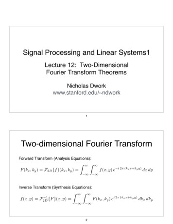
Illustration of DecompositionΦ3fα3f α1Φ1 α2Φ2 α3Φ3oα1α2Φ2Φ1Yao Wang, NYU-PolyEL5123: Fourier Transform4
Decomposition Ortho-normal basis function 1, u1 u2 ( x, u1 ) * ( x, u2 )dx 0, u1 u2 ForwardF (u ) f ( x),) ( x, u ) f ( x) *( x, u )dxdProjection off(x) onto (x,u) Inverse f ( x) F (u ) ( x, u )du Yao Wang, NYU-PolyRepresenting f(x) as sum of (x,u) for all u, with weightF(u)EL5123: Fourier Transform5
Fourier Transform Basis function ( x, u ) ej 2 ux, u , . Forward TransformF (u ) F{ f ( x)} f ( x)e j 2 ux dxd Inverse Transform f ( x) F {F (u )} F (u )e j 2 ux du 1 Yao Wang, NYU-PolyEL5123: Fourier Transform6
Important Transform Pairsf ( x) 1 f ( x) e j 2 f0 xF (u ) (u )F (u ) (u f 0 )1f ( x) cos(2 f 0 x) F (u ) (u f 0 ) (u f 0 ) 21 (u f 0 ) (u f 0 ) f ( x) sin( 2 f 0 x) F (u ) 2j 1, x x0f ( x) 0, otherwiseF (u ) sin( 2 x0u ) 2 x0 sinc(2 x0u ) usin( t )where, sinc(t ) tDerive the last transform pair in classYao Wang, NYU-PolyEL5123: Fourier Transform7
FT of the Rectangle Functionsin( 2 x0u )sin( t )F (u ) 2 x0 sinc(2 x0u ) where, sinc(t ) u tf(x)-1f(x)x0 11-2xx0 22xNote first zero occurs at u0 1/(2 x0) 1/pulse-width, other zeros are multiples of this.Yao Wang, NYU-PolyEL5123: Fourier Transform8
IFT of Ideal Low Pass Signal What is f(x)?F(u)-u0Yao Wang, NYU-Polyu0uEL5123: Fourier Transform9
Representation of FT Generally, both f(x) and F(u) are complex Two representationsF (u ) R(u ) jI (u )– Real and Imaginary– Magnitude and PhaseF (u ) A(u )e j (u ) , whereA(u ) R(u ) 2 I (u ) 2 , (u ) tan 1I (u )R (u(u )II(u)F(u)Φ(u) RelationshipR(u) RR (u ) A(u ) cos (u ),) I (u ) A(u ) sini (u ) Power spectrumP (u ) A(u ) F (u ) F (u ) F (u )2Yao Wang, NYU-Poly*EL5123: Fourier Transform210
What if f(x) is real? Real world signals f(x) are usually real F(u) is still complex,complex but has special propertiesF * (u ) F ( u )R (u ) R( u ), A(u ) A( u ), P(u ) P ( u ) : even functionI (u ) I ( u ),) (u ) ( u ) : odd functionYao Wang, NYU-PolyEL5123: Fourier Transform11
Property of Fourier Transform Duality Linearityf (t ) F (u )F (t ) f ( u )F a1 f1 ( x) a2 f 2 ( x) a1 F{ f1 ( x)} a2 F{ f 2 ( x)} ScalingS liF af ( x) aF{ f ( x)} Translationf ( x x0 ) ConvolutionF (u )e j 2 x0u ,f ( x)e j 2 u0 x F (u u0 )f ( x) g ( x) f ( x ) g ( )d f ( x) g ( x) F (u )G (u )We will review convolution later!Yao Wang, NYU-PolyEL5123: Fourier Transform12
Two Dimension Fourier Transform Basis functions ( x, y; u , v) e j ( 2 ux 2 vyy ) e j 2 ux e j 2 vyy , u , v , . Forward – TransformF (u, v) F { f ( x, y )} f ( x, y )e j 2 (ux vy ) dxdy Inverse – Transformf ( x, y ) F {F (u , v)} 1 F (u , v)ej 2 ( ux vy )dudv PropertyPt– All the properties of 1D FT apply to 2D FTYao Wang, NYU-PolyEL5123: Fourier Transform13
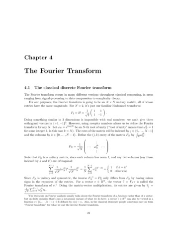
Example 1f ( x, y ) sin 4 x cos 6 yf(x,y)F {sin 4 x} sin 4 xe j 2 (ux vy ) dxdy sin 4 xe j 2 ux dx e j 2 vy dy sin 4 xe j 2 ux dx (v)1( (u 2) (u 2)) (v)2j1 ( (u 2, v) (u 2, v))2j , x y 0where ( x, y ) ( x) ( y ) 0, otherwiseuF(u,v)v1Likewise, F{cos 6 y} ( (u, v 3) (u , v 3))2Yao Wang, NYU-PolyEL5123: Fourier Transform14
Example 2f ( x, y ) sin( 2 x 3 y ) 1 j ( 2 x 3 y ) j ( 2 x 3 y )e e2j F e j ( 2 x 3 y ) e j ( 2 x 3 y ) e j 2 ( xu yv ) dxdy e j 2 x e j 2 ux dx e j 3 y e j 2 yv dy33 (u 1) (v ) (u 1, v )223Likewise, F e j ( 2 x 3 y ) (u 1, v )2Thereforeh f , F sin( 2 x 3 y ) 33 1 (u 1, v ) (u 1, v ) 22 2j [X,Y] meshgrid(-2:1/16:2,-2:1/16:2);[XY] meshgrid( 2:1/16:2 2:1/16:2);f sin(2*pi*X 3*pi*Y);imagesc(f); colormap(gray)Truesize, axis off;uF(u,v)vYao Wang, NYU-PolyEL5123: Fourier Transform15
Important Transform Pairs1 (u f x , v f y ) (u f x , v f y ) sin( 2 f x x 2 f y y ) 2j1 (u f x , v f y ) (u f x , v f y ) cos(2 f x x 2 f y y ) 22D rectangulargfunction 2D sinc functionYao Wang, NYU-PolyEL5123: Fourier Transform16
Properties of 2D FT (1) LinearityF a1 f1 ( x, y ) a2 f 2 ( x, y ) a1 F{ f1 ( x, y )} a2 F{ f 2 ( x, y )} Translationf ( x x0 , y y0 ) f ( x , y ) e j 2 ( u 0 x v 0 y ) F (u , v)e j 2 ( x0 u y 0 v ),F (u u0 , v v0 ) Conjugationf * ( x, y ) Yao Wang, NYU-PolyF * ( u , v)EL5123: Fourier Transform17
Properties of 2D FT (2) Symmetryf ( x, y ) is real F (u , v) F ( u , v) Convolution– Definition of convolutionf ( x, y ) g ( x, y ) f ( x , y ) g ( , )d d – Convolution theoryf ( x, y ) g ( x, y ) F (u , v)G (u , v)We will describe 2D convolution later!Yao Wang, NYU-PolyEL5123: Fourier Transform18
Separability of 2D FT and SeparableSignal Separability of 2D FTF2 { f ( x, y )} Fy {Fx { f ( x, y )}} Fx {Fy { f ( x, y )}}– where Fx, Fy are 1D FT along x and y.– one can do 1DFT for each row of original image, then1D FT along each column of resulting image Separable Signal– f(x,y) fx(x)fy(y)– F(u,v)( ) Fx((u)F) y((v),) where Fx(u) Fx{fx(x)}, Fy(u) Fy{fy(y)}– For separable signal, one can simply compute two 1Dtransforms!Yao Wang, NYU-PolyEL5123: Fourier Transform19
Example 1f ( x, y ) sin(3 x) cos(5 y )f x ( x) sin((3 x) f y ( y ) cos(5 y ) 1 (u 3 / 2) (u 3 / 2) 2j1Fy (v) (v 5 / 2) (v 5 / 2) 2Fx (u ) F (u , v) Fx(u ) Fy (v) 535 1 35353 (u , v ) (u , v ) (u , v ) (u , v ) 4j 22222222 uvYao Wang, NYU-PolyEL5123: Fourier Transform20
Example 2 1, x x0 , y y0f ( x, y ) 0, otherwiseF (u , v) 4 x0 y0 sinc(2 x0u ) sinc(2 y0 v)x2ux0 2y0 1-111vy-22w/ logrithmic mappingYao Wang, NYU-PolyEL5123: Fourier Transform21
Rotation Let x r cos , y r sin , u cos , v sin . 2D FT in polar coordinate (r(r, θ) and (ρ(ρ, Ø)F ( , ) 0 2 0f (r , )e j 2 ( r cos cos r sin sin ) rdrd f (r , )e j 2 r cos( )rdrd Propertyf (r , 0 ) Yao Wang, NYU-PolyF ( , 0 )EL5123: Fourier Transform22
Example of RotationYao Wang, NYU-PolyEL5123: Fourier Transform23
Fourier Transform For Discrete TimeSequence (DTFT) One Dimensional DTFT– f(n) is a 1D discrete time sequence– Forward TransformF (u ) f ( n )e j 2 unF(u)) isF(i periodici di iin u, withith periodi dof 1n – InverseITransformTf1/ 2f ( n) 1 / 2Yao Wang, NYU-PolyF (u )e j 2 un duEL5123: Fourier Transform24
Properties unique for DTFT Periodicity– F(u) F(u 1)– The FT of a discrete time sequence is onlyconsidered for u є (-½( ½ , ½),½) and u ½ is thehighest discrete frequency Symmetry for real sequencesf ( n) f * ( n) F (u ) F * ( u ) F (u ) F ( u ) F (u ) is symmetricYao Wang, NYU-PolyEL5123: Fourier Transform25
Example 1, n 0,1,., N 1;f ( n) 0, others F (u ) N 1 e j 2 nun 0 1 e j 2 uN1 e j 2 u e j ( N 1)usin 2 u ( N / 2)sin 2 u (1 / 2)f(n)0N-1N 10nThere are N/2 zeros in (0, ½], 1/N apartYao Wang, NYU-PolyEL5123: Fourier Transform26
Two Dimensional DTFT Let f(m,n) represent a 2D sequence Forward TransformF (u , v) f (m, n)e j 2 ( mu nv )m n Inverse Transform1/ 2f (m, n) 1/ 2 1 / 2 1 / 2F (u , v)e j 2 ( mu nv ) dudv Properties– Periodicity, Shifting and Modulation, EnergyConservationYao Wang, NYU-PolyEL5123: Fourier Transform27
PeriodicityF (u , v) f (m, n)e j 2 ( mu nv )m n F(u,v) is periodic in u, v with period 1, i.e.,for all integers k, l:– F(u k, v l) F(u, v) To see this considere j 2 ( m ( u k ) n ( v l )) e j 2 ( mu nv ) e j 2 ( mk nl ) e j 2 ( mu nv )In MATLAB, frequency scaling is such that 1 represents maximum freq u,v 1/2.Yao Wang, NYU-PolyEL5123: Fourier Transform28
Illustration of PeriodicityuLow frequencies1.0High frequencies0.5-1.0Yao Wang, NYU-Poly-0.500.5EL5123: Fourier Transform1.0v29
Fourier Transform TypesBand PassLow PassHigh Passuuu0.50.50.5v0.5-0.5-0.5v0.5 -0.5-0.5-0.50.5-0.5Non-zero frequency componentsYao Wang, NYU-PolyEL5123: Fourier Transform30v
Shifting and Modulation ShiftingF{ f (m m0 , n n0 )} k m m0 , l n n 0 m n f (m m0 , n n0 )e j 2 ( mu nv ) f (k , l )e j 2 (( k m0 )u (l n0 ) v )k l e j 2 ( m0u n0v ) f (k , l )e j 2 ( ku lv )k l f (m m0 , n n0 ) e j 2 ( m0u n0v ) F (u , v) Modulationej 2 ( mu0 nv0 )Yao Wang, NYU-Polyf (m, n) EL5123: Fourier TransformF (u u0 , v v0 )31
Energy Conservation Inner Product f , g f (m, n) g * (m, n)m n m n 0.5 0.5 f (m, n) G * (u , v)e j 2 ( mu nv ) dudv 0.5 0.5 f (m, n)e j 2 ( mu nv ) G * (u , v)dudv 0.5 0.5 m n 0.50.50.50.5 Energy Conservation 0.5 0.5 F (u , v)G * (u , v)dudv F , G m n Yao Wang, NYU-Poly2f (m, n) 0 .5 0 .5 0 .5 0 .52F (u , v) dudvEL5123: Fourier Transform32
Delta Function Fourier transform of a delta function F (u , v) (m, n)e j 2 ( mu nv ) 1m n (m, n) 1 Inverse Fourier transform of a deltafunctionf (m, n) 0.5 0.5 0 .5 0 .5 (u, v)e j 2 ( mu nv ) dudv 11 (u, v)Yao Wang, NYU-PolyEL5123: Fourier Transform33
Example21 1f (m, n) 000 1 2 1 mf(m,n)nF (u , v) 1e j 2 ( 1*u 1*v ) 2e j 2 ( 1*u 0*v ) 1e j 2 ( 1*u 1*v ) 1e j 2 (1*u 1*v ) 2e j 2 (1*u 0*v ) 1e j 2 (1*u 1*v ) j 2 sin 2 ue j 2 v j 4 sin 2 u j 2 sin 2 ue j 2 v j 4 sin 2 u (cos 2 v 1)Note: This signalgis low ppass in the horizontal direction,,and band pass in the vertical direction.Yao Wang, NYU-PolyEL5123: Fourier Transform34
Graph of F(u,v)204060800020 40 60 80 100Yao Wang, NYU-Polydu [-0.5:0.01:0.5];d [[-0.5:0.01:0.5];dv0 5 0 01 0 5]Fu abs(sin(2 * pi * du));Fv cos(2 * pi * dv);F 4 * Fu' * (Fv 1);mesh(du,( , dv,, F););colorbar;Imagesc(F);colormap(gray); truesize;EL5123: Fourier TransformUsing MATLAB freqz2:f [1,2,1;0,0,0;-1,-2,-1];freqz2(f)35
Linear Convolution Convolution of Continuous Signals– 1D convolution f ( x) h( x) f ( x )h( )d f ( )h( x )d Equalitiesf ( x) ( x) f ( x),)f ( x) ( x x0 ) f ( x x0 )– 2D convolutionf ( x, y ) h ( x, y ) Yao Wang, NYU-Polyf ( x , y )h( , )d d f ( , )h(x , y )d d EL5123: Fourier Transform36
Examples of 1D 0αx-1 1(2) 1 x 2h(-α)11αf(x)*h(x)1x1Yao Wang, NYU-Polyαxf(α)h(x-α)h(x-α)100(1) 0 x 1h(x)0αxEL5123: Fourier Transform2x37
Example of 2D Convolutiony1βh(x-α,y-β) 1yf(x,y)1xx(1) 0 x 1,0 x 1 0 y 1g(x,y) x*yy1h(x,y)1y2α1βx1f(x,y)*h(x,y)x-11αx(3) 1 x 2, 0 y 1g(x,y) (2-x)*y( ) (2 )*2Yao Wang, NYU-Polyx 1α(2) 0 x 1,0 x 1 1 y 2g(x,y) x*(2-y)h(x-α,y-β)yh(x-α,y-β)βy 1y-11βyh(x-α,y-β)1y-11x-1 xα(4) 1 x 2, 1 y 2g(x y) (2 x)*(2g(x,y) (2-x)(2-y)y)xEL5123: Fourier Transform38
Convolution of 1D Discrete Signals Definition of convolutionf ( n) * h( n) f ( n m) h( m) m f ( m) h( n m)m The convolution can be considered as the weightedaverage:– sample n-m is multiplied by h(m) Filtering: f(n) is the signal, and h(n) is the filter– Finite impulsepresponsep((FIR)) filter– Infinite impulse response (IIR) filter If the range of f(n) is (n0, n1), and the range of h(n) is(m0, m1),) then the range of f(n)*h(n)f(n) h(n) is (n0 m0, n1 m1)Yao Wang, NYU-PolyEL5123: Fourier Transform39
Example of 1D Discrete Convolutionh(n-m)f(n)03n-5nn0(a) n 0, g(n) 0mh(n)05h(n-m)nh(-m)0 nn-5m(b) 0 n 8, g(n) 0-50mh(n-m)f(n)*h(n)nn-50m(c) n 8,8 g(n) 080Yao Wang, NYU-PolynEL5123: Fourier Transform40
Convolution of 2D Discrete Signals Definition of convolution f (m, n) * h(m, n) f ( m k , n l ) h( k , l )k l f ( k , l ) h( m k , n l )k l Weighted average:– Pixel (m-k,n-l) is weighted by h(k,l) Range– If the range of f(mf(m, n) is m0 m m1, n0 n n1– If the range of h(m, n) is k0 m k1, l0 n l1,– Then the range of f(m, n)*h(m, n) ism0 k0 m m1 k1, n0 l0 n n1 l1Yao Wang, NYU-PolyEL5123: Fourier Transform41
Example of 2D Discrete Convolutionmkf(m,n)f(k,l)h(-1-k, -2-l)11nmh(m,n)lf(k l)h(2 k 1 l)f(k,l)h(2-k,1-l)k11lnf(m,n)*h(m,n) kk1h(-k,-l)12lYao Wang, NYU-PolylEL5123: Fourier Transform342
Go through an example in class for anarbitrary 3x3 (non-symmetric) filterYao Wang, NYU-PolyEL5123: Fourier Transform43
Separable Filtering A filter is separable if h(x, y) hx(x)hy(y) orh(m n) hx(m)hy(n).h(m,(n) Matrix representationTH hx hy– Where hx and hy are column vectors Example 1 0 1 1 H 2 0 2 2 1 0 1 hx hTy 1 0 1 1 Yao Wang, NYU-PolyEL5123: Fourier Transform44
DTFT of Separable Filter Previous example 1 0 1 1 H 2 0 2 2 1 0 1 hx hTy 1 0 1 1 Recognizing that the filter is separable 1 10 1 Fy (v) 1e j 2 v 0 ( 1)e j 2 v 2 j sin 2 v2 1 Fx(u ) 1e j 2 u 2 e j 2 u 2 2 cos 2 uF (u, v) Fx(u ) Fy (v) 4 j (1 cos 2 u ) sin 2 vYao Wang, NYU-PolyEL5123: Fourier Transform45
Separable Filtering If H(m,n) is separable, the 2D convolution canbe accomplished by first applying 1D filteringalong each row using hy(n), and then applying1D filtering to the intermediate result along eachcolumn using the filter hx(n) Proof f (m, n) * h(m, n) f (m k , n l )hx (k )hy (l )kl f (m k , n l )hy (l ) hx (k )k l g y (m k , n)hx (k )k ( f (m, n) * hy (n)) * hx (m)Yao Wang, NYU-PolyEL5123: Fourier Transform46
Go through an example of filtering usingseparable filter in classYao Wang, NYU-PolyEL5123: Fourier Transform47
Computation Cost Suppose– The size of the image is M*NM N.– The size of the filter is K*L. Non-separableNbl filtfilteringi– Each pixel: K*L mul; K*L – 1 add.– Total: M*N*K*L mul; M*N*(K*L-1) add.– When M N, K L M2K2 mul M2(K2-1) add.Yao Wang, NYU-PolyEL5123: Fourier Transform48
Computation Cost Separable:––––––––Each pixel in a row: L mul; L-1L 1 add.Each row: N*L mul; N*(L-1) add.M rows: M*N*L mul; M*N*(L-1) add.Each pixel in a column: K mul; K-1 add.Each column: M*K mul; M*(K-1) add.N columns: N*M*K mul; N*M*(K-1) add.Total: M*N*(K L) mul; M*N*(K L-2) add.When MM N,N KK L:L 2M2K mul; 2M2(K-1) add. Significant savings if K (and L) is large!Yao Wang, NYU-PolyEL5123: Fourier Transform49
Boundary Treatment When assuming theimage values outside agiven image are zero, thefiltered values in theboundary are affected byassumed zero valuesadversely ForF betterb tt results,lt usesymmetric extension((mirror image)g ) to fill theoutside image values200200 205203203200200 205203203195195 200200200200200 205195195200200 205195195Actual image pixelsYao Wang, NYU-PolyEL5123: Fourier TransformExtended pixels50
Computer implementation of convolution Boundary treatment– An image of size MxN convolving with a filter of size KxL will yield animage of size (M K-1,N L-1)– If the filter is symmetric, the convolved image should have extraboundary of thickness K/2 on each side– Filtered values in the outer boundary of K/2 pixels depend on theextended pixel values– For simplicity, we can ignore the boundary problem, and process onlythe inner rows and columns of the image, leaving the outer K/2 rowsand L/2 columns unchanged (if filter is low-pass) or as zero (if filter ishigh-pass) RRenormalization:li ti– The filtered value may not be in the range of (0,255) and may not beintegers– Use two-passpoperationp First pass: save directly filtered value in an intermediate floating-point array Second pass: find minimum and maximum values of the intermediate image,renormalize to (0,255) and rounding to integers– F round((F1-fmin)*255/(fmax-fmin)) ToT displaydi l ththe unnormalizedli d iimage didirectly,tl use “i“imagesc(( )” functionftiYao Wang, NYU-PolyEL5123: Fourier Transform51
Sample Matlab Program% readin bmp filex imread('lena.bmp');[xh xw] size(x);y double(x);% define 2D filterh ones(5,5)/25;[hh hw] size(h);hhh (hh - 1) / 2;hhw (hw- 1) / 2;% linear convolution, assuming the filter is non-separable (although this example filter is separable)z y; %or z zeros(xhz zeros(xh,xw)xw) if not lowlow-passpass filterfor m hhh 1:xh - hhh,%skip first and last hhh rows to avoid boundary problemsfor n hhw 1:xw - hhw,%skip first and last hhw columns to avoid boundary problemstmpy 0;for k -hhh:hhh,for l -hhw:hhw,tmpv tmpv y(m - k,n – l)* h(k hhh 1, l hhw 1);%h(0 0) is stored in h(hhh 1%h(0,0)h(hhh 1,hhw 1)hhw 1)endendz(m, n) tmpv;%for more efficient matlab coding, you can replace the above loop withz(m,n) sum(sum(y(m-hhh:m hhh,n-hhw:n hhw).*h))endendYao Wang, NYU-PolyEL5123: Fourier Transform52
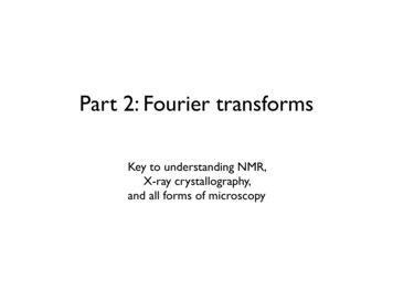
Results 1 11 1h 25 1 11 1 1 1 1 1 1 1 1 1 1 1 1 1 1 1 1 1 1 1 f(m,n)Yao Wang, NYU-Polyg(m,n)EL5123: Fourier Transform53
What if the filter is symmetric? Can youwrite a different MATLAB code that hasreduced computation time? MATLAB builtbuilt-inin functions– 1D filtering: conv– 2D filtering: conv2– Computing DTFT: freqz, freqz2Yao Wang, NYU-PolyEL5123: Fourier Transform54
Convolution Theorem Convolution Theoremf *h F H, f h ProofF *Hg (m, n) f (m, n) * h(m, n) f (m k , n l )h(k , l )klFT on both sidesG (u , v) f (m k , n l )h(k , l )e j 2 ( mu nv )m , n k ,l f (m k , n l )e j 2 (( m k )u ( n l ) v ) h(k , l )e j 2 ( ku lv )m , n k ,l f (m k , n l )e j 2 (( m k )u ( n l ) v ) h(k , l )e j 2 ( ku lv )m,nk ,l f (m' , n' )e j 2 ( m 'u n 'v ) h(k , l )e j 2 ( ku lv )m ', n 'k ,l F (u , v) H (u , v)Yao Wang, NYU-PolyEL5123: Fourier Transform55
Explanation of Convolutionin the Frequency Domainh(x)f(x)- /2 /2x- /4/F(u)( )-1/ g(x) f(x)*h(x) /4xxG(u) F(u)H(u)H(u)1/ Yao Wang, NYU-Polyu-2/ 2/ EL5123: Fourier Transformu-1/ u1/ 56
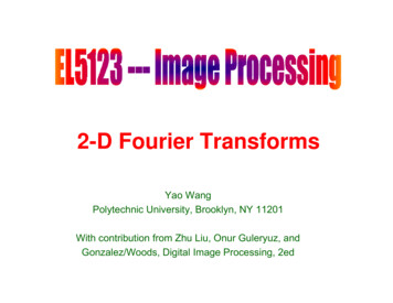
Example Given a 2D filter, show the frequency response. Apply to a givenimage, show original image and filtered image in pixel and freq.domain 1 11 1h 25 1 1Yao Wang, NYU-Poly1 1 1 1 1 1 1 1 1 1 1 1 1 1 1 1 1 1 1 1 EL5123: Fourier Transform57
1 11 1h 25 1 1Yao Wang, NYU-Poly1 1 1 1 1 1 1 1 1 1 1 1 1 1 1 1 1 1 1 1 EL5123: Fourier Transform58
Matlab Program Usedx imread('lena256.bmp');figure(1); imshow(x);f double(x);ff abs(fft2(f));figure(2); imagesc(fftshift(log(ff 1))); colormap(gray);truesize;axis off;h ones(5,5)/9;hf abs(freqz2(h));figure(3);imagesc((log(hf 1)));colormap(gray);truesize;axis off;y conv2(f, is off;yf abs(fft2(y));figure(5);imagesc(fftshift(log(yf 1)));colormap(gray);truesize;axis off;Yao Wang, NYU-PolyEL5123: Fourier Transform59
1 1 1 1 H1 0 0 0 3 1 1 1 Yao Wang, NYU-PolyEL5123: Fourier Transform60
Filter Design Given desired frequency response of the filterHd(u,v) Perform an inverse transform to obtain thedesired impulse response hd(m,n). When Hd(u,v) is band limited, hd(m,n) is infinitelylong Truncate hd(m,n)(m n) to yield a realizable h(mh(m,n)n) Will distort the original frequency response Better approach is to apply a well designedwindow function over the specified frequencyresponse.Yao Wang, NYU-PolyEL5123: Fourier Transform61
Use of Window Function in Filter DesignHd(u)H (u)uhd(x) Hw(u)uwindowfunctionw(x)h (x)uhw (x) xxHamming window w( x) 0.54 0.46 cos(2 Yao Wang, NYU-PolyEL5123: Fourier Transformxx), 0 x XX62
Homework1. Letf ( x, y ) sin 2 f 0 ( x y ), h( x, y ) sin(2 f c x) sin(2 f c y ) 2 xyFindFid theh convolvedl d signalil g(x,( y)) f(x,f( y)) * h(x,h( y)) ffor theh ffollowingll itwo cases:a) f0/2 fc f0; and b) f0 fc 2f0.Hint: do the filtering in the frequency domain. Explain whathappened by sketching the original signal, the filter, the convolutionprocess and the convolved signal in the frequency domain.2. Repeat the previous problem for11 2 {x, y} fc , h ( x, y ) 2 fc2 fc 0, otherwiseYao Wang, NYU-PolyEL5123: Fourier Transform63
Homework (cntd)3.For the three filters given below (assuming the origin is at the center):a) find their Fourier transforms (2D DTFT);b) sketch the magnitudes of the Fourier transformstransforms. You should sketch byhand the DTFT as a function of u, when v 0 and when v 1/2; also as afunction of v, when u 0 or ½. Also please plot the DTFT as a function ofboth u and v, usingg Matlab pplottingg function.c) Compare the functions of the three filters.In your calculation, you should make use of the separable property of the filterwhenever appropriate. If necessary, split the filter into several additiveterms such that each term can be calculated more efficiently. 1 1 1 1H1 1 1 1 9 1 1 1 Yao Wang, NYU-Poly 1 2 1 1 H2 2122 24 1 2 1 EL5123: Fourier Transform 1 2 1 1 H3 2122 24 1 2 1 64
Programming Assignment1.2.3.Write a Matlab or C-program for implementing filtering of a gray scaleimage. Your program should allow you to specify the filter with anarbitrary size (in the range of k0- k1, l0- l1), read in a gray scale image,and save the filtered image into another filefile. For simplicitysimplicity, ignore theboundary effect. That is, do not compute the filtered values for pixelsresiding on the image boundary. If the filter has a size of M x N, theboundary pixels are those in the top and bottom M/2 rows, and left andrightg most N/2 columns. You should pproperlyp y normalize the filtered imagegso that the resulting image values can be saved as 8-bit unsignedcharacters. Apply the filters given in the previous problem to a test image.Observe on the effect of these filters on your image. Note: you cannotuse the MATLAB conv2( ) function. In your report, include your MATLABcode the original test image and the images obtained with the threecode,filters. Write down your observation of the effect of the filters.Optional: Now write a convolution program assuming the filter isseparable. Your program should allow you to specify the horizontal andvertical filters,filters and call a 1D convolution sub-programsub program to accomplish the2D convolution. Note: you cannot use the MATLAB conv( ) function.Learn the various options of conv2( ) function in MATLAB using onlinehelp manual.Yao Wang, NYU-PolyEL5123: Fourier Transform65
Reading Gonzalez and Woods, Sec. 4.1 and 4.2,4 34.,3.4,4 33.5,5 33.55Yao Wang, NYU-PolyEL5123: Fourier Transform66
Continuous Fourier Transform (FT) – 1D FT (review) – 2D FT Fourier Transform for Discrete Time Sequence (DTFT) – 1D DTFT (review) – 2D DTFT Li C l tiLinear Convolution – 1D, Continuous vs. discrete signals (review) – 2D Filter Design Computer Implementation Yao Wa