Transcription
The relationship between Fourier and Mellintransforms, with applications to probabilityDave Collinsdcollins@unm.eduAbstractThe use of Fourier transforms for deriving probability densities of sumsand differences of random variables is well known. The use of Mellintransforms to derive densities for products and quotients of random variables is less well known. We present the relationship between the Fourierand Mellin transform, and discuss the use of these transforms in deriving densities for algebraic combinations of random variables. Results areillustrated with examples from reliability analysis.1IntroductionFor the purposes of this paper, we may loosely define a random variable (RV)as a value in some domain, say R, representing the outcome of a process basedon a probability law. An example would be a real number representing theheight in inches of a male chosen at random from a population in which heightis distributed according to a Gaussian (normal) law with mean 71 and variance25. Then we can say, for example, that the probability of the height of anindividual from the population being between 66 and 76 inches is about .68.For deriving such information about “nice” probability distributions (e.g.,the height distribution above), we integrate the probability densityfunction 211 x µ (pdf); in the case of the Gaussian the pdf is f x σ 2π exp 2 σ2 , whereµ is the mean and σ 2 is the variance.1A question that frequently arises in applications is, given RVs X, Y withdensities f x , g y , what is the density of the random variable X Y ? (Theanswer is not f x g y .) A less frequent but sometimes important questionis, what is the density of the product XY ? In this paper, after some briefbackground on probability theory, we provide specific examples of these questions and show how they can be answered with convolutions, using the Fourierand Mellin integral transforms. In fact (though we will not go into this level1 In this paper “nice” means RVs whose range is Rn , with finite moments of all orders,and which are absolutely continuous with respect to Lebesgue measure, which implies thattheir pdfs are smooth almost everywhere and Riemann integrable. We will only deal with nicedistributions.1
of detail), using these transforms one can, in principle, compute densities forarbitrary rational functions of random variables [15].1.1TerminologyTo avoid confusion, it is necessary to mention a few cases in which the terminology used in probability theory may be confusing: “Distribution” (or “law”) in probability theory means a function that assigns a probability 0 p 1 to every Borel subset of R; not a “generalizedfunction” as in the Schwartz theory of distributions. For historical reasons going back to Henri Poincaré, the term “characteristic function” in probability theory refers to an integral transform of a pdf,not to what mathematicians usually refer to as the characteristic function.For that concept, probability theory uses “indicator function”, symbolizedI; e.g., I 0,1 x is 1 for x 0, 1 and 0 elsewhere. In this paper we willnot use the term “characteristic function” at all. We will be talking about pdfs being in L1 R , and this should be takenin the ordinary mathematical sense of a function on R which is absolutelyintegrable. More commonly, probabilists talk about random variables being in L1 , L2 , etc., which is quite different—in terms of a pdf f , it meansthat x f x dx, x 2f x dx, etc. exist and are finite. It would requirean excursion into measure theory to explain why this makes sense; suffice it to say that in the latter case we should really say something like“L1 Ω, F, P ”, which is not at all the same as L1 R .2Probability backgroundFor those with no exposure to probability and statistics, we provide a briefintuitive overview of a few concepts. Feel free to skip to the end if you arealready familiar with this material (but do look at the two examples at the endof the section).Probability theory starts with the idea of the outcome of some process, whichis mapped to a domain (e.g., R) by a random variable, say X. We will ignorethe underlying process and just think of x R as a “realization” of X, with aprobability law or distribution which tells us how much probability is associatedwith any interval a, b R. “How much” is given by a number 0 p 1.Formally, probabilities are implicitly defined by their role in the axiomsof probability theory; informally, one can think of them as degrees of belief(varying from 0, complete disbelief, to 1, complete belief), or as ratios of thenumber of times a certain outcome occurs to the total number of outcomes (e.g.,the proportion of coin tosses that come up heads).A probability law on R can be represented by its density, or pdf, which isa continuous function f x with the property that the probability of finding x2
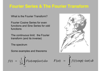
in a, b is P x a, b a f x dx. The pdf is just like a physical density—itgives the probability “mass” per unit length, which is integrated to measurethe total mass in an interval. Note the defining characteristics of a probabilitymeasure on R:b1. For any a, b , 02. P x 3. if a, b , c, d P x a, b 1.1. , then P x a, b c, d P x a, b P x c, d .From these properties and general properties of the integral it follows that if ff x dx 1.is a continuous pdf, then f x 0 and are also discrete random variables,Though we don’t need them here, therewhich take values in a countable set as opposed to a continuous domain. Forexample, a random variable representing the outcome of a process that countsthe number of students in the classroom at any given moment takes values onlyin the nonnegative integers. There is much more to probability, and in particulara great deal of measure-theoretic apparatus has been ignored here, but it is notnecessary for understanding the remainder of the paper.The Gaussian or normal density was mentioned in section 1. We say thatX N µ, σ 2 if it is distributed according to a normal law with mean or averageµ and variance σ 2 . The mean µ determines the center of the normal pdf, whichis symmetric; µ is also the median (the point such that half the probability massis above it, half below), and the mode (the unique local maximum of the pdf). Ifthe pdf represented a physical mass distribution over a long rod, the mean µ isthe point at which it would balance. The variance is a measure of the variabilityor “spread” of the distribution. The square root of the variance, σ, is called thestandard deviation, and is often used because it has the same unit of measureas X.Formally, given any RV X with pdf f , its mean is µ xf x dx (the average of x over the support of the distribution, weighted by the probabilitydensity). This is usually designated by E X , the expectation or expected valuex µ 2 f x dx (the weightedof X. The variance of X is E X µ 2 average of the squared deviation of x from its mean value).Figure 1 plots the N 71, 25 density for heights mentioned in Section 1. Thecentral vertical line marks the mean, and the two outer lines are at a distanceof one standard deviation from the mean. The definite integral of the normalpdf can’t be solved in closed form; an approximation is often found as follows:It is easy to show that if X N µ, σ 2 , then Xσ µ N 0, 1 ; also from theproperties of a probability measure, for any random variable X,P aXb P Xb P X a .It therefore suffices to have a table of values for PXb for theN 0, 1 distribution. (Viewed as a function of b, P b is called the cumulativedistribution function.) Such tables are found in all elementary statistics books,and give, e.g., P 66 X 76 .682.3
0.080.060.040.025060708090100Figure 1: N 71, 25 pdf for the distribution of heightsMany applications use random variables that take values only on 0, , forexample to represent incomes, life expectancies, etc. A frequently used modelfor such RVs is the gamma distribution with pdff x 1xα 1 e xΓ α β αβif x 0, 0 otherwise.(Notice that aside from the constant Γ α1 β α , which normalizes f so it integratesto 1, and the extra parameter β, this is the kernel of the gamma function Γ α 0 xα 1 e x dx, which accounts for the name.) Figure 2 shows a gamma(4, 2)pdf (α 4, β 2). Because a gamma density is never symmetric, but skewed tothe right, the mode, median and mean occur in that order and are not identical.For an incomes distribution this means that the typical (most likely) income issmaller than the “middle” income which is smaller than the average income (thelatter is pulled up by the small number of people who have very large incomes).Independence is profoundly important in probability theory, and is mainlywhat saves probability from being “merely” an application of measure theory.For the purposes of this paper, an intuitive definition suffices: two randomvariables X, Y are independent if the occurrence or nonoccurrence of an eventX a, b does not affect the probability of an event Y c, d , and vice versa.Computationally, the implication is that “independence means multiply”. E.g.,if X, Y are independent,P X a,b &Y c,d P X a,b P Y c,d .In this paper, we will only consider independent random variables.4
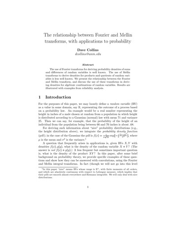
0.120.100.080.060.040.025101520Figure 2: gamma(4, 2) pdfExtending the example with which we began, suppose we consider heightsof pairs of people from a given population, where each member of the pair ischosen at random, so we can assume that their heights are independent RVsX, Y . Then for any given pair x, y we can ask, for example, about theprobability that both 66x76 and 66y76. This requires a joint orbivariate densityf x, y of X and Y . Using the “independence means multiply”rule above and taking limits as the interval sizes go to 0, it should be fairlyobvious that f x, y fX x fY y , where fX and fY are the densities of X andY . It follows thatP X 66,71 & Y71 66,7166By substituting ,readily seen thatbfX x dxa71fX x dx fY 71fY y dy71f x, y dxdy. 666666for either of the intervals of integration, it is also f by dy abx, y dxdyfX x dx. aAnd it follows that by “integrating out” one of the variables from the jointdensity f x, y , we recover the marginal density of the other variable: f x, y dx fY y .This is true whether or not X and Y are independent.Figure 3 illustrates this. The 3-D plot is a bivariate standard normal density,the product of two N 0, 1 densities. On the right is the marginal density of Y ,5
fY y ,which results from aggregating the density from all points x corresponding to a given y—i.e., integrating the joint density along the line Y y parallelto the x-axis. (The marginal density fY y is N 0, 1 , as expected.) Later, indiscussing convolution, we will see that it is also useful to integrate the jointdensity along a line that is not parallel to one of the coordinate axes.1.0Density0.520.0-20y-10x-212Figure 3: Bivariate normal pdf f x, y , with marginal density fY y 2.1ExamplesWith this background, here are two examples illustrating the need to computedensities for sums and products of RVs.Example 1 (Sum of random variables): Suppose you carry a backupbattery for a cellphone. Both the backup and the battery in the phone, whenfully charged, have a lifetime that is distributed according to a gamma lawf x gamma α, β , α 25, β .2, where x is in hours; αβ 5 hours is themean (average) life and αβ 2 1 is the variance. This density is shown in Figure4; it looks similar to a bell-shaped Gaussian, but it takes on only positive values.2What is the probability that both batteries run down in less than 10 hours? Toanswer questions like this we need the distribution of the sum of the randomvariables representing the lifetimes of the two batteries. E.g., if the lifetimes of2 Another difference: The Gaussian, as we know, is in the Schwartz class; the gamma pdfis not, since it is not C at the origin.6
the two batteries are represented by X gamma 25, .2 , Y gamma 25, .2 ,integrating the density of X Y from 0 to 10 will give the probablity that bothbatteries die in 10 hours or less.0.40.30.20.1246810Figure 4: gamma(25, .2) pdf for Battery lifeExample 2 (Product of random variables): The drive ratio of a pair ofpulleys connected by a drive belt is (roughly) the ratio of the pulley diameters,so, e.g., if the drive ratio is 2, the speed is doubled and the torque is halved fromthe first pulley to the second. In practice, the drive ratio is not exact, but isa random variable which varies slightly due to errors in determining the pulleydimensions, slippage of the belt, etc.Figure 5 shows an example: suppose a motor is turning the left-hand driveshaft at 800 rpm, which is connected to another shaft using a sequence of twobelt and pulley arrangements. The nominal drive ratios are 2 and 1.5; thusthe shaft connected to the pulley on the right is expected to turn at 2400 rpm(2 1.5 800).Suppose the motor speed is taken to be constant, and we are told in the manufacturer’s specifications that the first drive ratio is 2 .05 and the second is 1.5 .05. Given only this information, we might model the drive ratiosas uniform random variables, which distribute probability evenly over a finiteinterval; if the interval is a, b , the uniform a, b pdf is f x b 1 a I a,b x . Sothe two drive ratios in this case are given by RVs X uniform 1.95, 2.05 andY uniform 1.45, 1.55 . If the reliability of the system requires that the speedof the driven shaft be within a certain tolerance, then we need to know theprobability distribution describing the actual speed of the driven shaft. Thiswill be answered by computing the probability density for the product XY .7
Figure 5: Product of random variables: Belt and pulley drive3Transforms for sums of random variablesSuppose that the RV X has pdf fX x and Y has pdf fY y , and X and Yare independent. What is the pdf fZ z of the sum Z X Y ? Considerthe transformation ψ : R2R2 given by ψ x, y x, x y x, z . If wecan determine the joint density fXZ x, z , then the marginal density fZ z R fXZ x, z dx. The transformation ψ is injective with ψ 1 x, z x, z x and has Jacobian identically equal to 1, so we can use the multivariate changeof variable theorem to conclude that fZ z fXZ x, z dx RfXY ψ 1 x, z dx RfXY x, z x dxRfX x fY z R fX fY by the independence of X and Yx dxz .The next-to-last line above is intuitive: it says that we find the densityfor Z X Y by integrating the joint density of X, Y over all points where8
Y Z, i.e., where Y Z X. Figure 6 illustrates this for z R f 1 z g z dz is the integral of the joint density fXY x, y over the line y 1 x.X Figure 6: Integration path for f g 1 R f 1: f g 1 fX x fY y 1 z g z dz along the line y 1 x In general, computation of the convolution integral is difficult, and may beintractable. It is often simplified by using transforms, e.g., the Fourier transform:fX fY ξ fX ξ fY ξ The transform is then inverted to get fZ z .As an example, consider the gamma α, β pdf, whose Fourier transform isgiven by:Rx1xα 1 e β e 2πiξx dxαΓ α β 9 1 2πiξβ1xα 1 e x β dxαΓ α β Rα1β ΓαΓ α β α1 2πiξβ
112πiξβ αThere is a trick here in passing from the first to the second line. Recall thatthe kernel of the gamma α, β pdf integrates to Γ α β α ; Then notice that theβ pdf, which therefore integratesintegrand is the kernel of a gamma α, 1 2πiξβ αβto Γ α 1 2πiξβ .Thus the Fourier transform of the convolution of two independent gamma α, β RVs is1fX fY ξ 1 2πiξβ 2αwhich by inspection is the Fourier transform of a gamma 2α, β random variable.This answers the question posed in Example 1: If X, Y gamma 25, .2 ,then X Y gamma 50, .2 . By integrating this numerically (using Mathematica) the probability that both batteries die in 10 hours or less is found tobe about .519.In practice, we don’t require the Fourier transform; we can use any integraltransform T with the convolution property Tf g Tf Tg . In particular, sincedensities representing lifetimes are supported on 0, , the Laplace transformLf s 0 exp st f t dt, s R, is often used in reliability analysis.Note that the convolution result is extensible; it can be shown by inductionthat the Fourier transform of the pdf of a sum of n independent RVs X1 Xnwith pdfs f1 , . . . , fn is given by3 f1 fn ξ f1 ξ fn ξ 4 Transforms for products of random variablesWe now motivate a convolution for products, derive the Mellin transform fromthe Fourier transform, and show its use to compute products of random variables. This requires a digression into algebras on spaces of functions.4.1Convolution algebra on L1 R The general notion of an algebra is a collection of entities closed under operations that “look like” addition and multiplication of numbers. In the context offunction spaces (in particular L1 R , which is where probability density functions live) functions are the entities, addition and multiplication by scalars havethe obvious definitions, and we add an operation that multiplies functions.For linear function spaces that are complete with respect to a norm (Banachspaces4 ) the most important flavor of algebra is a Banach algebra [2, 12], with3 An application of this result is the famous central limit theorem, which says that undervery general conditions, the average of n independent and identically distributed random variables with any distribution whatsoever converges to a Gaussian distributed random variableas n . See [8], p. 114 ff., for a proof.4 If the norm is given by an inner product, the Banach space is a Hilbert space.10
the following properties ( is the multiplication operator, which is undefined forthe moment, λ is a scalar, and k is the norm on the space):i) fg h ii) fgh iii) fg hiv) λ fg v) k fgk fg h fg fh fg fh λf gf λg k f kk g kWe can’t use the obvious definition of multiplication to define an algebraover L1 R , because f, g L1 R does not imply f g L1 R . For example,one can verify that f x 1 e x is in L1 R (in fact, it is a pdf), butπ x 2 R fx 2 dx .Since L1 is not closed under ordinary multiplication of functions, we need adifferent multiplication operation, and convolution is the most useful possibility.To verify closure, if f, g L1 R ,kf gk R f y f RR RR R R R Ry x g x dx dyx g x dxdy fy fz dz g x dx by the substitution z x dy g x dx by Fubini’s theorem y xk f k g x dxk f kk g k .This also verifies property (v), the norm condition, and is sometimes calledYoung’s inequality.5 The remainder of the properties are easily verified, as wellas the fact that the convolution algebra is commutative: f g g f. 4.2 A product convolution algebraConsider the operator T : f x T -transformed functions byk f kT f0f ex for fex dx5 This f0L1 R . Define a norm for1y dyyis one of two different results that are called Young’s ’s inequality.11
where the last expression follows from the substitution y ex . Note thatf L1 R does not imply finiteness of the T -norm; for example, the pdf e x isin L1 R , but 0 e y y1 dx does not converge. This is also true for many otherpdfs, including the Gaussian.In order to salvage the T -norm for a function space that includes pdfs, weuse a modified version, the Mc -norm defined byk f kMc f 0x xc 1 dxwhere c is chosen to insure convergence for the class of functions we are interestedin. All pdfs f x satisfy 0 f x dx , and nice ones decay rapidly at infinityfor p 1; therefore k f kMc if c 1 for f in theso 0 xp f x dx class of “nice” pdfs.We can define a convolution for T -transformed functions by transformingthe functions in the standard convolution f g x f x u g u du: fg z : Tf f T g ex where z exex u g eu du0 f1elog z log w g elog w dww0 f z g w 1 dw.w w0(The next-to-last line follows from the substitutions z ex , w eu ). This iscalled the Mellin convolution. It is, like the Fourier convolution, commutative:f g g f.Now for fixed c R let Mc R be the space of functions on 0, withfinite Mc -norm. Using the obvious definitions of addition and multiplication byscalarsand the convolution for multiplication of functions, it can be shown that Mc R , , is a Banach algebra. Verifying closure under addition andscalar multiplication, and properties (i)–(iv), involves simple computations. Theproof of property (v) and closure under is lengthy, and we also need to provethat Mc R is a Banach space relative to the Mc -norm, i.e., that any Cauchysequence of functions with finite Mc -norms converges to a function with finiteMc -norm. We omit these here; for detailed proofs, see [5].4.3The Mellin transform, and its relation to the FouriertransformIf f Mc Rare in M 1, for all c a, b , we will say that f M a,b R (our “nice” pdfsR ). Then we define the Mellin transform of f with argument12
s C asF s M f s fu us 1 du0Re s b. (It is easy to show that if the integral converges forwhere as c R, it converges for s c it, t R . The subscript on M is usuallyomitted, with the assumption that the integral converges for the given s.For F s M f s , the inverse Mellin transform isf x M 1 M f x 12πi Fc i c is x s dsThe condition that the inverse exists is that F s x s is analytic in a stripa, b i , i such that c a, b [5].The Mellin transform can be derived from the Fourier transformfˆ ξ f x e 2πiξx dx R using the transformation T and the substitution ξ T f ξ Tf η c2πi f ex e 2πiξx dx f ex e η c x dx f y e η c log y 1 dyy0 f0 f for cη c2πifor real c 0: 0with the substitution y ex1y y c y η dyyy y η 1 dyfor fy f y y c .0 c(An aside on the substitution ξ η2πi: The factor of 2π is a consequenceof the way we define the Fourier transform. In statistics, and in many engineerf x eiξx dx (essentiallying texts, the Fourier transform is defined as fˆ ξ measuring frequency in radians per time unit instead of cycles per time unit),which simplifies the derivation of the Mellin transform from the Fourier transform. For a summary of the different ways the Fourier transform and its inverseare represented, see [13], Appendix D.)The same technique is used to derive the Mellin inversion formula from theFourier inversion: f y T 1 fˆ y fˆ ξ e2πi log y ξ dξ 13
f y y c fˆ η c e η c log y dη2πic i c i1 f η yc y η dη2πi c i2πi c i1 f η y η dη2πi c i2πi f y .c i12πiwith the substitution ξ In some cases the transformation T provides an easier way to invert Mellintransforms, through the use of Fourier inversion techniques.For computing the pdf of a product of random variables, the key result willbe that the Mellin transform of a Mellin convolution is the product of the Mellintransforms of the convolved functions:M fg s 0 0 0 0 fz1dw z s 1 dz g w ww0 f z z s 1 dz g w 1 dwww0 fy y s 1 ws 1 w dy g w 0 fby Fubini’s theorem1dwwsubstituting y zwy y s 1 dy g w ws 1 dw0M f s M g s As with the Fourier convolution, this result is extensible; it can be shown byinduction that the Mellin transform of the Mellin convolution of of f1 , . . . , fn isgiven byM f14.4 fn s M f1 s M fn s (1)Products of random variablesSuppose we have random variables X, Y with pdfs fX , fY , and the productR2Z XY is to be determined. Consider the transformation ψ : R26x, z . Except at x 0, ψ is injective withgiven by ψ x, y x, xy x, y ψ 1 x, z x, z x and the Jacobian of ψ 1 is J 1 ψ1 x 1 ψ1 z6 This ψ2 x 1 ψ2 1z 1 0 1 x2 1 1.xxcan be handled gracefully using Lebesgue integration theory, but here we ignore theproblem.14η c2πi
Then using the multivariate change of variable theorem, the marginal densityof Z is computed from the joint density of X and Z asfZ z fXZ x, z dx R 1fXY ψ 1 x, z dxxR z 1fXY x, dxx xR z 1dx by the independence of X and YfX x fYx xRfX fY z .This is precisely the Mellin convolution of fX and fY . In principle, thisplus the extensibility result (1) provides a way of finding product densities forarbitrary numbers of random variables.Note that the Mellin transform is defined only for functions supported on thepositive half-line R , whereas many pdfs (e.g., the Gaussian) do not satisfy thisrequirement. For such cases, the problem can be worked around by separatingthe positive and negative parts of the pdf; see [15] for details.4.5An exampleAs a simple illustration of the use of the Mellin transform, we use the belt andpulley example (Example 2, p. 7). Recall that X uniform 1.95, 2.05 , Y uniform 1.45, 1.55 and we seek the pdf of the product XY .The problem can be simplified by using the fact that a uniform α, β randomvariable can be expressed as αα β U , where U is a uniform 0, 1 randomvariable with pdf I 0,1 x . In this case, X 1.95 .1U, Y 1.45 .1U . ThenXY 2.8275 .34U .01U 2 . Since we already know how to compute sums, theproblem reduces to finding the pdf for the product of two uniform 0, 1 randomvariables.For Z U 2 , the Mellin convolution evaluates tofZ z fX x fY R1 1dxx log x z z z1dxx x1log z ,0The bounds for the integration come from x15 z1.1 and y1x z.
This result can also be obtained as M 1 M fU s 2 x , where fU is thepdf of U . We have11xs 1 dx M fU s s0so we needM 11z s2 12πi z s dss2c i c iwhich evaluates to the same result after an exercise in using the residue theoremof complex analysis.In this simple case of the product of two uniform(0,1) RVs it is easier tocompute the Mellin convolution directly; but the use of Mellin transforms allowscomputation of the pdf for a product of n uniform(0,1) RVs almost as easily,n 1 log z (another exercise in residue calculus).yieldingn 1 !The difficulty of either directly integrating the Mellin convolution or inverting a product of Mellin transforms escalates quickly for less simple distributionssuch as the gamma or normal. In particular, whereas the transforms of Fourierconvolutions of pdfs can often be evaluated by inspection (possibly using tables),this is not the case for Mellin transforms, though extensive tables do exist [3].This seems to be a consequence of the fact that sums of RVs often have pdfswith mathematical forms similar to the individual RVs (e.g., a sum of normalRVs is normal), unlike products of RVs (e.g., the uniform example above).The reader is referred to [15] for realistic examples, which are too lengthyto reproduce here.5SummaryWe have presented some background on probability theory, and two examplesmotivating the need to compute probability density functions for sums andproducts of random variables. The use of the Fourier or Laplace transform toevaluate the convolution integral for the pdf of a sum is relatively straightforward. The use of the Mellin transform to evaluate the convolution integral forthe pdf of a product is less well-known, but equally straightforward, at least intheory.In practice, though the use of Fourier or Laplace transforms for sums ofrandom variables is widely used and explained in every advanced statistics text,the Mellin transform remains obscure. Aside from Epstein’s seminal paper of1948 [9], there was a brief flurry of activity in the 1960s and 70s by Springerand Thompson (e.g., [16]) culminating in Springer’s book [15]. Current texts inprobability and statistics, however, do not mention the Mellin transform, andits appearance in current literature is rare.To some extent the relative lack of interest in products of random variablesis due to the lesser importance of products in applications. It probably also is16
a consequence of the greater difficulty of working with the integrals involved—particularly the fact that inverting the Mellin transform requires a strong knowledge of complex variable methods, which are not part of the standard graduatecurriculum in statistics. Nevertheless, it seems worthwhile for any statistician todevelop at least a nodding acquaintance with Mellin transform methods. Mathematicians and engineers will also find interesting applications (see the furtherreading below).5.1Further reading[11] is a nice summary of all the transform techniques used in probability theory.[15] is the ultimate reference on transform techniques for algebraic combinationsof random variables.For the use of integral transforms to compute sums of random variables, seeany graduate textbook on probability and statistics, e.g., [4, 6].[1], [19], [11], and [15] all cover the Mellin transform, the last two in theprobability context. [3] contains an extensive table of Mellin transforms (aswell as Fourier, Laplace, and other transforms). [5] contains a very completetreatment of properties of the Mellin transform, with proofs.[1] and [19] provide considerable depth on integral transforms generally, oriented towards applied mathematics. A more abstract view is provided by [20],which includes a treatment of integral transforms of (Schwartz) distributions.The algebraic properties of Fourier and Mellin transforms are (briefly) workedout in a series of exercises in [8] (ex. 9–15, pp. 41–43; ex. 2, p. 88; ex. 3, p.103). For the more algebraically inclined, one can develop an abstract theory ofconvolution and Fourier analysis on groups. See [7], “Appendix: functions ongroups” for an elementary introduction, or [14] for a full treatment.Probability and statistics is only one application area for the Mellin transform, and it is not the most important. The Mellin transform is used in com
and differences of random variables is well known. The use of Mellin transforms to derive densities for products and quotients of random vari-ables is less well known. We present the relationship between the Fourier and Mellin transform, and discuss the use of these transforms in deriv-ing