Transcription
1APPLICATIONS AND REVIEW OF FOURIER TRANSFORM/SERIES(David Sandwell, Copyright, 2004)(Reference – The Fourier Transform and its Application, second edition, R.N. Bracewell,McGraw-Hill Book Co., New York, 1978.)Fourier analysis is a fundamental tool used in all areas of science and engineering. The fastfourier transform (FFT) algorithm is remarkably efficient for solving large problems. Nearlyevery computing platform has a library of highly-optimized FFT routines. In the field of Earthscience, fourier analysis is used in the following areas:Solving linear partial differential equations (PDE’s):Gravity/magneticsLaplace 2 Φ 0Elasticity (flexure)Biharmonic 4 Φ 0Heat ConductionDiffusion 2Φ - δ Φ/ δt 0Wave PropagationWave 2Φ - δ2Φ/ δt2 0Designing and using antennas:Seismic arrays and streamersMultibeam echo sounder and side scan sonarInterferometers – VLBI – GPSSynthetic Aperture Radar (SAR) and Interferometric SAR (InSAR)Image Processing and filters:Transformation, representation, and encodingSmoothing and sharpeningRestoration, blur removal, and Wiener filterData Processing and Analysis:High-pass, low-pass, and band-pass filtersCross correlation – transfer functions – coherenceSignal and noise estimation – encoding time seriesIn this remote sensing course we will use fourier analysis to understand and evaluate apertures(antennas and telescopes) as well as to filter images. Fourier analysis deals with complex numbers so perhaps it is time to dust off your book onadvanced calculus. Here is a very brief review of the things you’ll need. A complex numberz x iy is composed of real and imaginary numbers. Remember i 1 . Functions can havereal and imaginary components as well. For example a general, complex-valued function of areal variable is f (x) u(x) iw(x) . The most important complex-valued function for this isin θ . After a little algebra it is easydiscussion is the complex exponential function e iθ cos θ iθ iθiθ iθe ee eto show that cosθ and sin θ . This is the level of math you’ll need to22i understand fourier analysis.
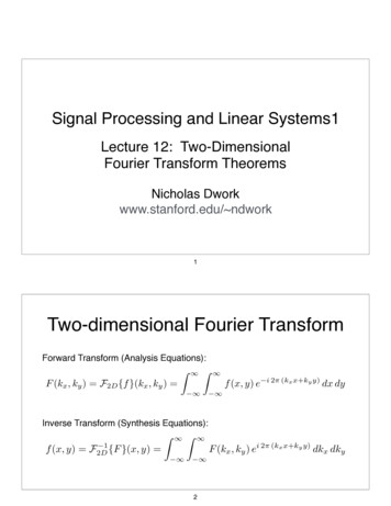
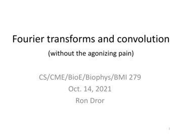
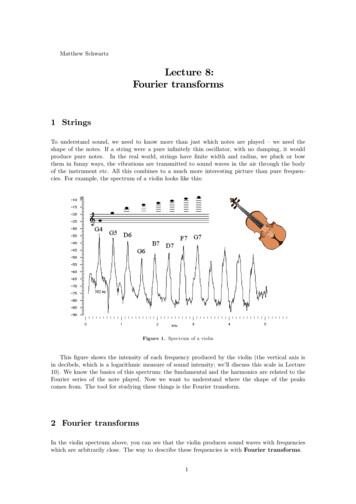
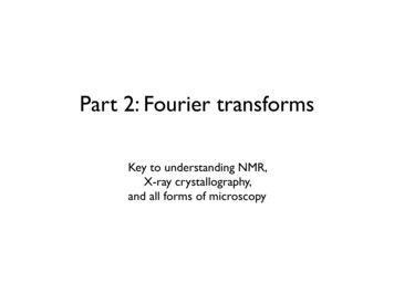
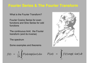
2Definitions of fourier transforms in 1-D and 2-DThe 1-dimensional fourier transform is defined as: F(k) f(x)e i2 πkxdxF(k) ℑ[ f(x)]- forward transform f(x) F(k)ei2 πkxdkf(x) ℑ 1[ F(k)] - inverse transform where x is distance and k is wavenumber where k 1/λ and λ is wavelength. These equationsare more commonly written in terms of time t and frequency ν where ν 1/T and T is the period.The 2-dimensional fourier transform is defined as: F(k) f (x)e i 2 π (k x )d 2xF(k) ℑ2 [ f (x)] f (x) F(k)ei2π (k x )d 2kf (x) ℑ2 1 [ F(k)] where x (x, y) is the position vector, k (kx, ky) is the wavenumber vector, and(k . x) kx x ky y.The next two page show some examples of fourier transform pairs. These figures were takenfrom Bracewell [1978].
3
4
5Fourier sine and cosine transformsAny function f(x) can be decomposed into odd O(x) and even E(x) components.f(x) E(x) O(x)E(x) 1[ f(x) f( x)]2O(x) 1[ f(x) f( x)]2 F(k) f(x)e i2 πkxdx e iθ cosθ isin θ F(k) f(x)cos(2π kx)dx i f(x)sin(2πkx)dx odd part cancels even part cancels F(k) 2 E(x)cos(2π kx)dx 2i O(x)sin(2πkx)dxoocosine transformsine transformYou have probably seen fourier cosine and sine transforms, but it is better to use the complexexponential form.
6
7Properties of fourier transformsThe following are some important properties of fourier transforms that you should derive foryourself at least once. You’ll find derivations in Bracewell. Once you have derived andunderstand these properties, you can treat them as tools. Very complicated problems can besimplified using these tools. For example, when solving a linear partial differential equation, oneuses the derivative property to reduce the differential equation to an algebraic equation.similarity propertyshift propertydifferentiation propertyconvolution propertyℑ[ f(ax)] ℑ[ f(x - a)] e i2πka F(k) df ℑ i2πk F(k) dx ℑ f (u)g( x -u )du F(k)G( k) - Rayleigh' s theorem1 k F a a 2 2 f (x) dx F(k) dk- - Note: These properties are equally valid in 2-dimensions or even n-dimensions. The propertiesalso apply to discrete data. See Chapter 18 in Bracewell.
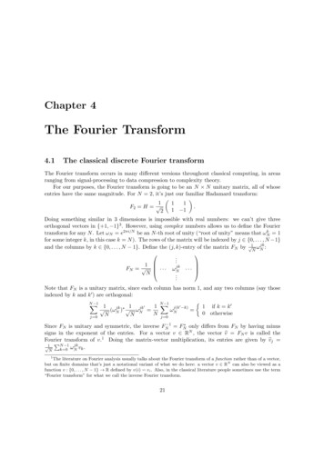
8Fourier seriesMany geophysical problems areconcerned with a small area on thesurface of the Earth.yWWW - width of areaL - length of areaΔyΔxLxThe coefficients of the 2-dimensional Fourier series are computed by the following integration.Fnm 1LWL W mn f (x, y)exp i2π L x W y dydxo oThe function is reconstructed by the following summations over the fourier coefficients. f (x, y) mn Fn m mn exp i2π x y LW The finite size of the area leads to a discrete set of wavenumbers kx m/L, ky n/W and adiscrete set of fourier coefficients Fnm. In addition to the finite size of the area, geophysical datacommonly have a characteristic sampling interval Δx and Δy.I L/Δx- number of points in the x-directionJ W/ Δy - number of points in the y-directionThe Nyquist wavenumbers is kx 1/(2 Δx) and ky 1/(2 Δy) so there is a finite set of fouriercoefficients -I/2 m I/2 and -J/2 n J/2. Recall the trapesoidal rule of integration.L oI 1f (x)dx f (xi )Δx where xi iΔx.i 0L of (x)dx L I 1f (xi )I i 0
9The discrete forward and inverse fourier transform are:1F IJmnfi j I 1 J 1j fI/2ii o j oJ/2mn Fn I / 2 m J / 2 mn exp i2π i j I J ij exp i2π m n IJ The forward and inverse discrete fourier transforms are almost identical sums so one can use thesame computer code for both operations.
2 Definitions of fourier transforms in 1-D and 2-D The 1-dimensional fourier transform is defined as: where x is distance and k is wavenumber where k 1/λ and λ is wavelength.These equations are more commonly written in terms of time t and frequency ν where ν 1/T and T is the period. The