Transcription
Lecture NotesControl System Engineering-IIVEER SURENDRA SAI UNIVERSITY OF TECHNOLOGY BURLA, ODISHA, INDIADEPARTMENT OF ELECTRICAL ENGINEERINGCONTROL SYSTEM ENGINEERING-II (3-1-0)Lecture NotesSubject Code: CSE-IIFor 6th sem. Electrical Engineering & 7th Sem. EEE Student1
DISCLAIMERCOPYRIGHT IS NOT RESERVED BY AUTHORS. AUTHORS ARE NOT RESPONSIBLEFOR ANY LEGAL ISSUES ARISING OUT OF ANY COPYRIGHT DEMANDS AND/ORREPRINT ISSUES CONTAINED IN THIS MATERIALS. THIS IS NOT MEANT FOR ANYCOMMERCIAL PURPOSE & ONLY MEANT FOR PERSONAL USE OF STUDENTSFOLLOWING SYLLABUS. READERS ARE REQUESTED TO SEND ANY TYPINGERRORS CONTAINED, HEREIN.2
Department of Electrical Engineering,CONTROL SYSTEM ENGINEERING-II (3-1-0)MODULE-I (10 HOURS)State Variable Analysis and Design: Introduction, Concepts of State, Sate Variables and State Model,State Models for Linear Continuous-Time Systems, State Variables and Linear Discrete-TimeSystems, Diagonalization, Solution of State Equations, Concepts of Controllability and Observability,Pole Placement by State Feedback, Observer based state feedback control.MODULE-II (10 HOURS)Introduction of Design: The Design Problem, Preliminary Considerations of Classical Design,Realization of Basic Compensators, Cascade Compensation in Time Domain(Reshaping the RootLocus), Cascade Compensation in Frequency Domain(Reshaping the Bode Plot),Introduction to Feedback Compensation and Robust Control System Design.Digital Control Systems: Advantages and disadvantages of Digital Control, Representation ofSampled process, The z-transform, The z-transfer Function. Transfer function Models and dynamicresponse of Sampled-data closed loop Control Systems, The Z and S domain Relationship, StabilityAnalysis.MODULE-III (10 HOURS)Nonlinear Systems: Introduction, Common Physical Non-linearities, The Phase-plane Method: BasicConcepts, Singular Points, Stability of Nonlinear System, Construction of Phase-trajectories, TheDescribing Function Method: Basic Concepts, Derivation of Describing Functions, Stability analysisby Describing Function Method, Jump Resonance, Signal Stabilization.Liapunov‟s Stability Analysis: Introduction, Liapunov‟s Stability Criterion, The Direct Method ofLiapunov and the Linear System, Methods of Constructing Liapunov Functions for NonlinearSystems, Popov‟s Criterion.MODULE-IV (10 HOURS)Optimal Control Systems: Introduction, Parameter Optimization: Servomechanisms, Optimal ControlProblems: State Variable Approach, The State Regulator Problem, The Infinite-time RegulatorProblem, The Output regulator and the Tracking Problems, Parameter Optimization: Regulators,Introduction to Adaptive Control.BOOKS[1]. K. Ogata, “Modem Control Engineering”, PHI.[2]. I.J. Nagrath, M. Gopal, “Control Systems Engineering”, New Age International Publishers.[3]. J.J.Distefano, III, A.R.Stubberud, I.J.Williams, “Feedback and Control Systems”, TMH.[4]. K.Ogata, “Discrete Time Control System”, Pearson Education Asia.3
MODULE-IState space analysis.State space analysis is an excellent method for the design and analysis of control systems.The conventional and old method for the design and analysis of control systems is thetransfer function method. The transfer function method for design and analysis had manydrawbacks.Advantages of state variable analysis. It can be applied to non linear system. It can be applied to tile invariant systems. It can be applied to multiple input multiple output systems. Its gives idea about the internal state of the system.State Variable Analysis and DesignState: The state of a dynamic system is the smallest set of variables called state variables such thatthe knowledge of these variables at time t to (Initial condition), together with the knowledge of inputfor 𝑡0 , completely determines the behaviour of the system for any time 𝑡 𝑡0 .State vector: If n state variables are needed to completely describe the behaviour of a given system,then these n state variables can be considered the n components of a vector X. Such a vector is calleda state vector.State space: The n-dimensional space whose co-ordinate axes consists of the x1 axis, x2 axis,. xnaxis, where x1 , x2 ,. xn are state variables: is called a state space.State ModelLets consider a multi input & multi output system is havingr inputs 𝑢1 𝑡 , 𝑢2 𝑡 , . 𝑢𝑟 (𝑡)m no of outputs 𝑦1 𝑡 , 𝑦2 𝑡 , . 𝑦𝑚 (𝑡)n no of state variables 𝑥1 𝑡 , 𝑥2 𝑡 , . 𝑥𝑛 (𝑡)Then the state model is given by state & output equationX t AX t BU t state equationY t CX t DU t output equationA is state matrix of size (n n)B is the input matrix of size (n r)C is the output matrix of size (m n)4
D is the direct transmission matrix of size (m r)X(t) is the state vector of size (n 1)Y(t) is the output vector of size (m 1)U(t) is the input vector of size (r 1)(Block diagram of the linear, continuous time control system represented in state space)𝐗 𝐭 𝐀𝐗 𝐭 𝐁𝐮 𝐭𝐘 𝐭 𝐂𝐗 𝐭 𝐃𝐮 𝐭STATE SPACE REPRESENTATION OF NTH ORDER SYSTEMS OF LINEARDIFFERENTIAL EQUATION IN WHICH FORCING FUNCTION DOES NOT INVOLVEDERIVATIVE TERMConsider following nth order LTI system relating the output y(t) to the input u(t).𝑦 𝑛 𝑎1 𝑦 𝑛 1 𝑎2 𝑦 𝑛 2 𝑎𝑛 1 𝑦1 𝑎𝑛 𝑦 𝑢Phase variables: The phase variables are defined as those particular state variables which areobtained from one of the system variables & its (n-1) derivatives. Often the variables used isthe system output & the remaining state variables are then derivatives of the output.Let us define the state variables as𝑥1 𝑦𝑥2 𝑑𝑦 𝑑𝑥 𝑑𝑡 𝑑𝑡𝑥3 𝑑𝑦 𝑑𝑥2 𝑑𝑡𝑑𝑡 𝑥𝑛 𝑦 𝑛 1 5𝑑𝑥𝑛 1𝑑𝑡
From the above equations we can write𝑥1 𝑥2𝑥2 𝑥3 𝑥𝑛 1 𝑥𝑛𝑥𝑛 𝑎𝑛 𝑥1 𝑎𝑛 1 𝑥2 𝑎1 𝑥𝑛 𝑢Writing the above state equation in vector matrix formX t AX t Bu t00Where 𝑋 , 𝐴 0𝑥𝑛 𝑛 1 𝑎𝑛𝑥1𝑥21 0 0 1 0 0 𝑎𝑛 1 𝑎𝑛 2 .00 1 𝑎1𝑛 𝑛Output equation can be written asY t CX t𝐶 1 0 . 01 𝑛Example: Direct Derivation of State Space Model (Mechanical Translating)Derive a state space model for the system shown. The input is fa and the output is y.We can write free body equations for the system at x and at y.6
Freebody DiagramEquationThere are three energy storage elements, so we expect three state equations. The energystorage elements are the spring, k2, the mass, m, and the spring, k1. Therefore we chooseas our state variables x (the energy in spring k2 is ½k2x²), the velocity at x (the energy inthe mass m is ½mv², where v is the first derivative of x), and y (the energy in spring k 1 is½k1(y-x)² , so we could pick y-x as a state variable, but we'll just use y (since x is already astate variable; recall that the choice of state variables is not unique). Our state variablesbecome:Now we want equations for their derivatives. The equations of motion from the free bodydiagrams yieldor7
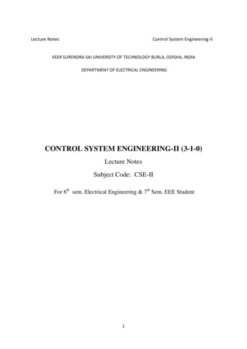
with the input u fa.Example: Direct Derivation of State Space Model (Electrical)Derive a state space model for the system shown. The input is ia and the output is e2.There are three energy storage elements, so we expect three state equations. Trychoosing i1, i2 and e1 as state variables. Now we want equations for their derivatives. Thevoltage across the inductor L2 is e1 (which is one of our state variables)so our first state variable equation isIf we sum currents into the node labeled n1 we getThis equation has our input (ia) and two state variable (iL2 and iL1) and the currentthrough the capacitor. So from this we can get our second state equationOur third, and final, state equation we get by writing an equation for the voltage acrossL1 (which is e2) in terms of our other state variablesWe also need an output equation:8
So our state space representation becomesState Space to Transfer FunctionConsider the state space system:Now, take the Laplace Transform (with zero initial conditions since we are finding atransfer function):We want to solve for the ratio of Y(s) to U(s), so we need so remove Q(s) from theoutput equation. We start by solving the state equation for Q(s)The matrix Φ(s) is called the state transition matrix. Now we put this into the outputequationNow we can solve for the transfer function:Note that although there are many state space representations of a given system, allof those representations will result in the same transfer function (i.e., the transferfunction of a system is unique; the state space representation is not).9
Example: State Space to Transfer FunctionFind the transfer function of the system with state space representationFirst find (sI-A) and the Φ (sI-A)-1 (note: this calculation is not obvious. Detailsare here). Rules for inverting a 3x3 matrix are here.Now we can find the transfer functionTo make this task easier, MatLab has a command (ss2tf) for converting from state spaceto transfer function. % First define state space system A [0 1 0; 0 0 1; -3 -4 -2]; B [0; 0; 1]; C [5 1 0]; [n,d] ss2tf(A,B,C,D)n 10
001.00001.00003.00002.00004.00005.0000d mySys tf tf(n,d)Transfer function:s 5---------------------s 3 2 s 2 4 s 3Transfer Function to State SpaceRecall that state space models of systems are not unique; a system has many state spacerepresentations. Therefore we will develop a few methods for creating state space modelsof systems.Before we look at procedures for converting from a transfer function to a state spacemodel of a system, let's first examine going from a differential equation to state space.We'll do this first with a simple system, then move to a more complex system that willdemonstrate the usefulness of a standard technique.First we start with an example demonstrating a simple way of converting from a singledifferential equation to state space, followed by a conversion from transfer function to statespace.Example: Differential Equation to State Space (simple)Consider the differential equation with no derivatives on the right hand side. We'll usea third order equation, thought it generalizes to nth order in the obvious way.For such systems (no derivatives of the input) we can choose as our n state variables thevariable y and its first n-1 derivatives (in this case the first two derivatives)11
Taking the derivatives we can develop our state space modelNote: For an nth order system the matrices generalize in the obvious way (A has ones above themain diagonal and the differential equation constants for the last row, B is all zeros with b0 in thebottom row, C is zero except for the leftmost element which is one, and D is zero)Repeat Starting from Transfer FunctionConsider the transfer function with a constant numerator (note: this is the same systemas in the preceding example). We'll use a third order equation, thought it generalizes tonth order in the obvious way.For such systems (no derivatives of the input) we can choose as our n state variables thevariable y and its first n-1 derivatives (in this case the first two derivatives)Taking the derivatives we can develop our state space model (which is exactly the sameas when we started from the differential equation).12
Note: For an nth order system the matrices generalize in the obvious way (A has onesabove the main diagonal and the coefficients of the denominator polynomial for the lastrow, B is all zeros with b0 (the numerator coefficient) in the bottom row, C is zero exceptfor the leftmost element which is one, and D is zero)If we try this method on a slightly more complicated system, we find that itinitially fails (though we can succeed with a little cleverness).Example: Differential Equation to State Space (harder)Consider the differential equation with a single derivative on the right hand side.We can try the same method as before:The method has failed because there is a derivative of the input on the right hand, andthat is not allowed in a state space model.Fortunately we can solve our problem by revising our choice of state variables.Now when we take the derivatives we get:13
The second and third equations are not correct, because ÿ is not one of the statevariables. However we can make use of the fact:The second state variable equation then becomesIn the third state variable equation we have successfully removed the derivative of theinput from the right side of the third equation, and we can get rid of the ÿ term using thesame substitution we used for the second state variable.The process described in the previous example can be generalized to systems withhigher order input derivatives but unfortunately gets increasingly difficult as the orderof the derivative increases. When the order of derivatives is equal on both sides, theprocess becomes much more difficult (and the variable "D" is no longer equal tozero). Clearly more straightforward techniques are necessary. Two are outlinedbelow, one generates a state space method known as the "controllable canonical form"and the other generates the "observable canonical form (the meaning of these termsderives from Control Theory but are not important to us).Controllable Canonical Form (CCF)Probably the most straightforward method for converting from the transferfunction of a system to a state space model is to generate a model in "controllablecanonical form." This term comes from Control Theory but its exact meaning is notimportant to us. To see how this method of generating a state space model works,consider the third order differential transfer function:We start by multiplying by Z(s)/Z(s) and then solving for Y(s) and U(s) in terms ofZ(s). We also convert back to a differential equation.14
We can now choose z and its first two derivatives as our state variablesNow we just need to form the outputFrom these results we can easily form the state space model:In this case, the order of the numerator of the transfer function was less than that ofthe denominator. If they are equal, the process is somewhat more complex. A resultthat works in all cases is given below; the details are here. For a general nth ordertransfer function:the controllable canonical state space model form isKey Concept: Transfer function to State Space (CCF)For a general nth order transfer function:the controllable canonical state space model form is15
Observable Canonical Form (OCF)Another commonly used state variable form is the "observable canonical form."This term comes from Control Theory but its exact meaning is not important to us.To understand how this method works consider a third order system with transferfunction:We can convert this to a differential equation and solve for the highest orderderivative of y:Now we integrate twice (the reason for this will be apparent soon), and collect termsaccording to order of the integral:Choose the output as our first state variableLooking at the right hand side of the differential equation we note that y q1 and wecall the two integral terms q2:soThis is our first state variable equation.16
Now let's examine q2 and its derivative:Again we note that y q1 and we call the integral terms q3:soThis is our second state variable equation.Now let's examine q3 and its derivative:This is our third, and last, state variable equation.Our state space model now becomes:In this case, the order of the numerator of the transfer function was less than that ofthe denominator. If they are equal, the process is somewhat more complex. A resultthat works in all cases is given below; the details are here. For a general nth ordertransfer function:the observable canonical state space model form is17
Key Concept: Transfer function to State Space (OCF)For a general nth order transfer function:the observable canonical state space model form is𝐂 Adj SI A 𝐁 SI A DSI ASI A is also known as characteristic equation when equated to zero. MATLab CodeTransfer Function to State Space(tf2ss)Y(s)s 32U(s) s 14s 56s 160num [1 0];den [1 14 56 160];[A,B,C,D] tf2ss(num,den)A -14 -56 -16010001018
B 100C 010D 0Concept of Eigen Values and Eigen VectorsThe roots of characteristic equation that we have described above are known as eigen valuesof matrix A.Now there are some properties related to eigen values and these properties are written belowAny square matrix A and its transpose AT have the same eigen values.Sum of eigen values of any matrix A is equal to the trace of the matrix A.Product of the eigen values of any matrix A is equal to the determinant of the matrix A.If we multiply a scalar quantity to matrix A then the eigen values are also get multiplied bythe same value of scalar.5. If we inverse the given matrix A then its eigen values are also get inverses.6. If all the elements of the matrix are real then the eigen values corresponding to that matrix areeither real or exists in complex conjugate pair.1.2.3.4.Eigen VectorsAny non zero vector 𝑚𝑖 that satisfies the matrix equation 𝜆𝑖 𝐼 𝐴 𝑚𝑖 0 is called the eigenvector of A associated with the eigen value 𝜆𝑖 ,. Where𝜆𝑖 , i 1, 2, 3, .n denotes the itheigen values of A.This eigen vector may be obtained by taking cofactors of matrix 𝜆𝑖 𝐼 𝐴 along any row &transposing that row of cofactors.19
DiagonalizationLet 𝑚1 , 𝑚2 , . . 𝑚𝑛 be the eigenvectors corresponding to the eigen value 𝜆1 , 𝜆2 , . . 𝜆𝑛respectively.Then 𝑀 𝑚1 𝑚2 𝑚𝑛 is called diagonalizing or modal matrix of A.Consider the nth order MIMO state modelX t AX t BU tY t CX t DU tSystem matrix A is non diagonal, so let us define a new state vector V(t) such thatX(t) MV(t).Under this assumption original state model modifies toV t 𝐴V t BU tY t CV t DU tWhere 𝑨 𝑴 𝟏 𝑨𝑴 𝑑𝑖𝑎𝑔𝑜𝑛𝑎𝑙 𝑚𝑎𝑡𝑟𝑖𝑥,𝑩 𝑴 𝟏 𝑩 ,𝑪 𝑪𝑴The above transformed state model is in canonical state model. The transformation describedabove is called similarity transformation.If the system matrix A is in companion form & if all its n eigen values are distinct, thenmodal matrix will be special matrix called the Vander Monde matrix.1𝜆1𝑉𝑎𝑛𝑑𝑒𝑟 𝑀𝑜𝑛𝑑𝑒 𝑚𝑎𝑡𝑟𝑖𝑥 𝑉 𝜆1𝑛 2𝜆1𝑛 11𝜆2 𝜆𝑛 22𝑛 1𝜆21 𝜆3 𝜆𝑛 2 3𝑛 1𝜆3 .1𝜆𝑛 𝑛 2𝜆𝑛𝜆𝑛 1𝑛𝑛 𝑛State Transition Matrix and Zero State ResponseWe are here interested in deriving the expressions for the state transition matrix and zero stateresponse. Again taking the state equations that we have derived above and taking theirLaplace transformation we have,20
Now on rewriting the above equation we haveLet [sI-A]-1 θ(s) and taking the inverse Laplace of the above equation we haveThe expression θ(t) is known as state transition matrix(STM).L-1.θ(t)BU(s) zero state response.Now let us discuss some of the properties of the state transition matrix.1. If we substitute t 0 in the above equation then we will get 1.Mathematically we can writeθ(0) 1.2. If we substitute t -t in the θ(t) then we will get inverse of θ(t). Mathematically we can writeθ(-t) [θ(t)]-1.3. We also another important property [θ(t)]n θ(nt).Computation of STN using Cayley-Hamilton TheoremThe Cayley–hamilton theorem states that every square matrix A satisfies its owncharacteristic equation.This theorem provides a simple procedure for evaluating the functions of a matrix.To determine the matrix polynomial𝑓 𝐴 𝑘0 𝐼 𝑘1 𝐴 𝑘2 𝐴2 𝑘𝑛 𝐴𝑛 𝑘𝑛 1 𝐴𝑛 1 Consider the scalar polynomial𝑓(𝜆) 𝑘0 𝑘1 𝜆 𝑘2 𝜆2 𝑘𝑛 𝜆𝑛 𝑘𝑛 1 𝜆𝑛 1 Here A is a square matrix of size (n n). Its characteristic equation is given by𝑞 𝜆 𝜆𝐼 𝐴 𝜆𝑛 𝑎1 𝜆𝑛 1 𝑎2 𝜆𝑛 2 𝑎𝑛 1 𝜆 𝑎𝑛 0If 𝑓 𝐴 is divided by the characteristic polynomial 𝑞 𝜆 , then𝑓 𝜆𝑅 𝜆 𝑄 𝜆 𝑞 𝜆𝑞 𝜆𝑓 𝜆 𝑄 𝜆 𝑞 𝜆 𝑅 𝜆 . . (1)Where 𝑅 𝜆 is the remainder polynomial of the form𝑅 𝜆 𝑎0 𝑎1 𝜆 𝑎2 𝜆2 𝑎𝑛 1 𝜆𝑛 1 (2)21
If we evaluate 𝑓 𝐴 at the eigen values 𝜆1 , 𝜆2 , . . 𝜆𝑛 , then 𝑞 𝜆 0 and we have fromequation (1) 𝑓 𝜆𝑖 𝑅 𝜆𝑖 ; 𝑖 1,2, . 𝑛 . . (3)The coefficients 𝑎0 , 𝑎1 , . . 𝑎𝑛 1 , can be obtained by successfully substituting𝜆1 , 𝜆2 , . . 𝜆𝑛 into equation (3).Substituting A for the variable 𝜆 in equation (1), we get𝑓 𝐴 𝑄 𝐴 𝑞 𝐴 𝑅 𝐴As 𝑞 𝐴 𝑖𝑠 𝑧𝑒𝑟𝑜, 𝑠𝑜 𝑓 𝐴 𝑅 𝐴 𝑓 𝐴 𝑎0 𝐼 𝑎1 𝐴 𝑎2 𝐴2 𝑎𝑛 1 𝐴𝑛 1𝑤 𝑖𝑐 𝑖𝑠 𝑡 𝑒 𝑑𝑒𝑠𝑖𝑟𝑒𝑑 𝑟𝑒𝑠𝑢𝑙𝑡.CONCEPTS OF CONTROLLABILITY & OBSERVABILITYState ControllabilityA system is said to be completely state controllable if it is possible to transfer thesystem state from any initial state X(to) to any desired state X(t) in specified finite time by acontrol vector u(t).Kalman‟s testConsider nth order multi input LTI system with m dimensional control vectorX t AX t BU tis completely controllable if & only if the rank of the composite matrix Qc is n.𝑸𝒄 𝑩 𝑨𝑩 𝑨𝒏 𝟏 𝑩ObservabilityA system is said to be completely observable, if every state X(to) can be completelyidentified by measurements of the outputs y(t) over a finite time interval(𝑡𝑜 𝑡 𝑡1 ).Kalman‟s testConsider nth order multi input LTI system with m dimensional output vectorX t AX t BU tY t CX t DU tis completely observable if & only if the rank of the observability matrix Qo is n.𝑸𝒐 [𝑪𝑻 𝑨𝑻 𝑪𝑻 𝑨𝑻22𝒏 𝟏 𝑻𝑪 ]
Principle of Duality: It gives relationship between controllability & observability. The Pair (AB) is controllable implies that the pair (AT BT ) is observable. The pair (AC) is observable implies that the pair (AT CT ) is controllable.Design of Control System in State SpacePole placement at State SpaceAssumptions: The system is completely state controllable. ƒ The state variables are measurable and are available for feedback. ƒ Control input is unconstrained.Objective:The closed loop poles should lie at 𝜇1 , 𝜇2 , . . 𝜇𝑛 which are their „desired locations‟Necessary and sufficient condition: The system is completely state controllable.Consider the systemX t AX t BU tThe control vector U is designed in the following state feedback form U -KXThis leads to the following closed loop systemX t A BK X t ACL X tThe gain matrix K is designed in such a way that𝑆𝐼 𝐴 𝐵𝐾 𝑆 𝜇1 𝑆 𝜇2 . . 𝑆 𝜇𝑛Pole Placement Design Steps:Method 1 (low order systems, n 3): Check controllability Define 𝐾 𝑘1 𝑘2 𝑘3 Substitute this gain in the desired characteristic polynomial equation𝑆𝐼 𝐴 𝐵𝐾 𝑆 𝜇1 𝑆 𝜇2 . . 𝑆 𝜇𝑛 Solve for 𝑘1 , 𝑘2 , 𝑘3 by equating the like powers of S on both sidesMATLab CodeFinding State Feedback gain matrix with MATLabMATLab code acker is based on Ackermann‟s formula and works for single input singleoutput system only.MATLab code place works for single- or multi-input system.23
ExampleConsider the system with state equationX tWhere010A 001 ,B 1 5 6 AX t BU t001By using state feedback control u -Kx, it is desired to have the closed –loop poles at𝜇1 2 𝑗4,𝜇2 2 𝑗4,𝜇3 10Determine the state feedback gain matrix K with MATLabA [0 1 0;0 0 1;-1 -5 -6];B [0;0;1];J [-2 i*4 -2-i*4 -10];k acker(A,B,J)k 199558A [0 1 0;0 0 1;-1 -5 -6];B [0;0;1];J [-2 i*4 -2-i*4 -10];k place(A,B,J)k 199.000055.00008.0000State Estimators or Observers One should note that although state feed back control is very attractive because of precisecomputation of the gain matrix K, implementation of a state feedback controller is possibleonly when all state variables are directly measurable with help of some kind of sensors. Due to the excess number of required sensors or unavailability of states for measurement, inmost of the practical situations this requirement is not met. Only a subset of state variables or their combinations may be available for measurements.Sometimes only output y is available for measurement.24
Hence the need for an estimator or observer is obvious which estimates all state variableswhile observing input and output.Full Order Observer : If the state observer estimates all the state variables, regardless ofwhether some are available for direct measurements or not, it is called a full orderobserver.Reduced Order Observer : An observer that estimates fewer than n'' states of thesystem is called reduced order observer.Minimum Order Observer : If the order of the observer is minimum possible then it iscalled minimum order observer.Observer Block DiagramDesign of an ObserverThe governing equation for a dynamic system (Plant) in statespace representation may bewritten as:X t AX t BU tY t CX tThe governing equation for the Observer based on the block diagram is shown below. Thesuperscript „ ‟ refers to estimation.𝑋 𝐴𝑋 𝐵𝑈 𝐾𝑒 (𝑌 𝑌)𝑌 𝐶𝑋25
Define the error in estimation of state vector as𝑒 (𝑋 𝑋)The error dynamics could be derived now from the observer governing equation and statespace equations for the system as:𝑒 (𝐴 𝐾𝑒 𝐶)𝑒𝑌 𝑌 𝐶𝑒The corresponding characteristic equation may be written as: 𝑆𝐼 (𝐴 𝐾𝑒 𝐶) 0You need to design the observer gains such that the desired error dynamics is obtained.Observer Design Steps:Method 1 (low order systems, n 3): Check the observability𝑘𝑒1Define 𝐾𝑒 𝑘𝑒2𝑘𝑒3Substitute this gain in the desired characteristic polynomial equation 𝑆𝐼 (𝐴 𝐾𝑒 𝐶) 𝑆 𝜇1 𝑆 𝜇2 . . 𝑆 𝜇𝑛Solve for 𝑘1 , 𝑘2 , 𝑘3 by equating the like powers of S on both sidesHere 𝜇1 , 𝜇2 , . . 𝜇𝑛 are desired eigen values of observer matrix.26
MODEL QUESTIONSModule-1Short Questions each carrying Two marks.1. The System matrix of a continuous time system, described in the state variable formisx 0 0A 0 y 10 1 2Determine the range of x & y so that the system is stable.2. For a single input systemX AX BUY CX010A ; B ; C 1 1 1 21Check the controllability & observability of the system.013. Given the homogeneous state space equation X X; 1 2Determine the steady state value 𝑋𝑠𝑠 lim𝑡 𝑋(𝑡) given the initial state value10X(0) . 104. State Kalman‟s test for observability.The figures in the right-hand margin indicate marks.5. For a system represented by the state equation X AXWhere010A 302 12 7 6Find the initial condition state vector X(0) which will excite only the modecorresponding to the eigenvalue with the most negative real part.[10]6. Write short notes on Properties of state transition matrix.[3.5]7. Investigate the controllability and observability of the following system:1 00𝑋 𝑋 𝑢; 𝑌 0 1 𝑋[8]0 218. Write short notes on[4 5](a) Pole placement by state feedback.(b) state transition matrix(c) MIMO systems(d) hydraulic servomotor(e) Principle of duality due to kalman9. A system is described by the following differential equation. Represent the system instate space:27
𝑑3 𝑋𝑑2 𝑋𝑑𝑋 3 4 4𝑋 𝑢1 𝑡 3𝑢2 𝑡 4𝑢3 (𝑡)𝑑𝑡 3𝑑𝑡 2𝑑𝑡and outputs are𝑦1 4𝑦2 𝑑2𝑋𝑑𝑡 2𝑑𝑋 3𝑢1𝑑𝑡 4𝑢2 𝑢3[8]10. Find the time response of the system described by the equation 1 10𝑋(𝑡) 𝑋 𝑢(t)0 21 1X 0 , u t 1, t 0011. (a) Obtain a state space representation of the systemC(s)U(s)10(s 2) s 3 3s 2 5s 15[14][7](b) A linear system is represented by 6 411 0𝑋 𝑋 𝑈;𝑌 𝑋 2 011 1(i) Find the complete solution for Y(t) when U(t) 1(t), 𝑋1 0 1, 𝑋2 0 0(ii) Draw a block diagram representing the system.[5 3]12. Discuss the state controllability of the system𝑋1 3 1 𝑋11 uX 21.54𝑋22Prove the conditions used.[3 4]13. If a continuous-time state equation is represented in discrete form asX[(K 1)T] G(T)X(KT) H(T) U(KT)Deduce the expressions for the matrices G(T) & H(T)Discretise the continuous-time system described by0 10𝑋 𝑋 𝑈;0 01Assume the sampling period is 2 secs.[5 4]14.(a) Choosing 𝑥1 current through the inductor[8]𝑥2 voltage across capacitor,determine the state equation for the system shownin fig below(b) Explain controllability and observability.15. A linear system is represented by 6 41𝑥 𝑥 u 2 0128[8]
1 0𝑥1 1(a)Find the complete solution for y(t) whenU(t) 1(t), 𝑥1 (0) 1 and 𝑥2 (0) 0(b) Determine the transfer function(c) Draw a block diagram representing the system[9 4 3]16.(a) Derive an expression for the transfer function of a pump controlled hydraulic system.State the assumption made.[8](b) Simulate a pneumatic PID controller and obtain its linearized transfer function.[8]17. Describe the constructional features of a rate gyro, explain its principle of operation andobtain its transfer function.[8]18. (a) Explain how poles of a closed loop control system can be placed at the desired pointson the s plane.[4](b) Explain how diagonalisation of a system matrix a helps in the study of controllabilityof control systems.[4]19. Construct the state space model of the system whose signal flow graph is shown in fig 2.[7]Y 20. (a)Define state of a system, state variables, state space and state vector. What are theadvantages of state space analysis?(b) A two input two output linear dynamic system is governed by012 1𝑋(𝑡) X(t) R(t) 2 30 11 0Y(t) X(t)1 1i)Find out the transfer function matrix.ii)Assuming 𝑋 0 0 find the output response Y(t) if0R(t) 3𝑡 for t 0𝑒21.(a) A system is described by 4 10𝑋(t) 0 3 1 X(t)00 2Diagonalise the above system making use of suitable transformation X PZ(b) Show how can you compute 𝑒 𝐴𝑡 using results of (a)22. Define controllability and observability and of control systems.23. A feed back system has a closed loop transfer function:29[5][5][5][8][7][4]
𝑌(𝑠)10𝑠 40 3𝑅(𝑠) 𝑠 𝑠 2 3𝑠Construct three different state models showing block diagram in each case.[5 3]24. Explain the method of pole placement by state-feedback. Find the matrix k [𝑘1 𝑘2 ]which is called the state feedback gain matrix for the closed loop poles to be located at -1.8 .j2.4 for the original system governed by the state equation:𝑋 010X 𝑈20.6 01[6]25.(a) From a system represented by the state equation𝑥 𝑡 𝐴 𝑥(𝑡)The response of 2𝑡1X(t) 𝑒 2𝑡 when x(0) 2 2𝑒 𝑡1And x(t) 𝑒 𝑡 when x(o) 1 𝑒Determine the system matrix A and the states transition matrix φ(t).(b) Prove non uniqueness of state space model.26.(a) Show the following system is always controllable010001 𝑥 0 𝑢𝑥 𝑡 0 𝑎3 𝑎2 𝑎 11(b) Explain the design of state observer.(c) Illustrate and explain pole placement by state feedback.30[12][4][4 4 4]
MODULE-IICOMPENSATOR DESIGNEvery control system which has been designed for a specific application shouldmeet certain performance specification. There are always some constraints which areimposed on the control system design in addi
Digital Control Systems: Advantages and disadvantages of Digital Control, Representation of Sampled process, The z-transform, The z-transfer Function. Transfer function Models and dynamic response of Sampled-data closed loop Control Systems, The Z and S domai