Transcription
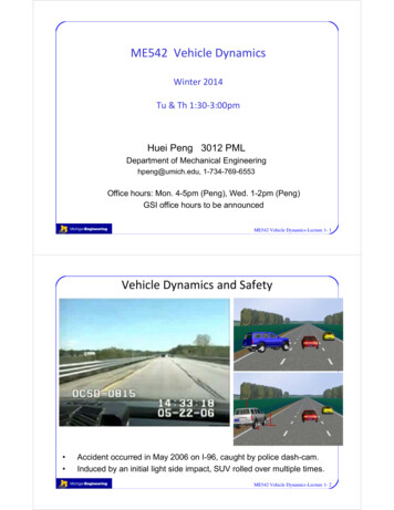
ME542 Vehicle DynamicsWinter 2014Tu & Th 1:30‐3:00pmHuei Peng 3012 PMLDepartment of Mechanical Engineeringhpeng@umich.edu, 1-734-769-6553Office hours: Mon. 4-5pm (Peng), Wed. 1-2pm (Peng)GSI office hours to be announcedME542 Vehicle Dynamics-Lecture 1- 1Vehicle Dynamics and Safety Accident occurred in May 2006 on I-96, caught by police dash-cam.Induced by an initial light side impact, SUV rolled over multiple times.ME542 Vehicle Dynamics-Lecture 1- 2
Lecture 1‐‐Introduction and Motivation(and administrative stuff) About this course––––Introduction and administrative informationMajor course contentGrading policyMATLAB/SIMULINK Review of rigid body dynamicsME542 Vehicle Dynamics-Lecture 1- 3Administrative Information Textbook (not required)– J.Y. Wong, Theory of Ground Vehicles, John Wiley &Sons, Inc, 4thedition, 2008. d‐0470170387.html) Course material will be made available on the Ctools site(PPT files should be downloaded and printed before thelectures, HW, solutions, example MATLAB programs willbe distributed using this site)ME542 Vehicle Dynamics-Lecture 1- 4
Course Requirements Prerequisites– Knowledge in Newtonian Dynamics (ME240 level) isessential– That of Automotive Engineering (ME458) andIntermediate Dynamics (ME440) are helpful but notrequired.– Familiarity with Matlab/Simulink, since Matlab/Simulinkis used extensively in the lecture examples andhomework assignments.ME542 Vehicle Dynamics-Lecture 1- 5Major course contentLec. /3234/8244/10254/15264/17274/224/25Lecture contentsIntroduction, motivationReview of Rigid Body DynamicsMATLAB‐SIMULINK reviewTire Models: Overview, Terminology, DefinitionsBrush Tire Model (Lateral)Brush Tire Model (Lateral)Brush Tire Model (Longitudinal)Combined‐Slip Tire Model(Lateral) Taut String Tire Model, Magic Formula Tire ModelOff‐road tire modelSteady‐State HandlingSteady‐State Handling: Understeering and OversteeringTransient HandlingLateral‐Yaw‐Roll modelLateral‐Yaw‐Roll modelFour‐Wheel SteeringMidterm (in class)Guest lecture: chassis control systemsOn‐Center Handling, Steady‐State And Transient Handling of ArticulatedVehiclesDriver‐vehicle interactionCross‐wind stabilityRide dynamics—Principle and Vibration Isolation and human perceptionRide dynamics—road excitationsRide dynamics—Quarter‐car suspension ModelRide dynamics—Quarter‐car suspension ModelRide dynamics—Bounce and Pitch ModelRide dynamics—Active SuspensionsSummaryFinal exam (4‐6pm)ME542 Vehicle Dynamics-Lecture 1- 6
Related Courses ME458 Automotive EngineeringEmphasizes the vehicle as an engineering system andreview design consideration associated with all majorsystems including the vehicle structure, powertrain,suspension, steering and braking. ME568 Vehicle Control SystemsCovers control issues for all major vehicle controlsystems including engine control, cruise control,ABS/traction control, four‐wheel steering, activesuspension and advanced control systems for IntelligentTransportation Systems.ME542 Vehicle Dynamics-Lecture 1- 7Grading Policy Grading:5‐6 HomeworkMidterm examFinal exam55%20%25% Homework: Must be handed in on the due date in class (on‐campusstudents) or uploaded to Ctools (distance learning students). Latehomework will be accepted up to 48 hours late with a 20% penalty foreach 24 hours (rounded up, i.e., 0 to 24 hours late 24 hours late). Allproblem sets (home work assignments) are to be completed on yourown. You may discuss homework assignments with your fellowstudents at the conceptual level, but must complete all calculations andwrite‐up, from scrap to final form, on your own. Verbatim copying ofanother student's work is forbidden. If you have any questions aboutthis policy, please do not hesitate to contact the instructor. Exams:Midterm: in class, Dynamics, Tire, HandlingFinal exam: 2 hours, Accumulative but more weight onHandling and RideME542 Vehicle Dynamics-Lecture 1- 8
MATLAB/SIMULINK 2 Vehicle Dynamics-Lecture 1- 9Getting a Copy of MATLAB/SIMULINKCAEN labsStudent ersion/Virtual Sitehttp://virtualsites.umich.edu/ME542 Vehicle Dynamics-Lecture 1- 10
MATLAB/SIMULINK Example MATLAB/SIMULINK programs will bedistributed, which you can freely use/modify. MATLAB is used for simple (usually linear) vehicledynamic simulations and analysis for this course. SIMULINK: A GUI based simulation program.Strength:– Realistic dynamic phenomenon such as nonlinearity,quantization, noise, switches, look‐up tables, delays,etc. can be simulated easily.– GUI makes it easy to recycle vehicle simulationmodulesME542 Vehicle Dynamics-Lecture 1- 11Review of Rigid Body Dynamics Vehicle Coordinate Systems Newton/Euler Formulation Lagrange FormulationME542 Vehicle Dynamics-Lecture 1- 12
Vehicle Coordinate System First step in deriving vehicle dynamic equations. The Society of Automotive Engineers (SAE) hasintroduced standard coordinates and notations fordescribing vehicle dynamicslateraly pitchxverticalyawzlongitudinalrollISO coordinate: x is the same but y and z are reversed.ME542 Vehicle Dynamics-Lecture 1- 13SAE Vehicle‐Fixed Coordinate System‐‐Symbols and DefinitionsAxisTranslationalVelocityxu (forward)AngularDisplacement AngularVelocityForceComponentMomentComponentp or (roll)FxMxq or (pitch)FyMyr or (yaw)FzMz/ˈfaɪ/yv (lateral) /ˈθiːtə/, US /ˈθeɪtə/zw (vertical) /ˈsaɪ/, /ˈpsaɪ/Pitch angle: the angle between x‐axis and the horizontal plane.Roll angle: the angle between y‐axis and the horizontal plane.Yaw angle: the angle between x‐axis and the X‐axis of a inertia frameME542 Vehicle Dynamics-Lecture 1- 14
Earth Fixed Coordinate and Vehicle SlipOXYZ fixed on Earth (does not turn with the vehicle)Course angle Heading angleSideslip angleIn the left figure,sideslip angle isnegative)tan OvuME542 Vehicle Dynamics-Lecture 1- 15Tire SlipSource: Wong page 7o:Z:X and Y axes:Tire camber angle:Center of tire contact patchPerpendicular to the ground plane.On the ground plane.Angle between the XZ plane and thewheel plane.ME542 Vehicle Dynamics-Lecture 1- 16
Ride/Handling DynamicsInvolves vehicle motions in several directionsSPRUNG G MASSverticalwheel rotationRIDE HANDLING ( ) ME542 Vehicle Dynamics-Lecture 1- 17Newton/Euler FormulationConsider a rigid body of mass m, with c.g. at point o,subject to N external forces.For unconstrained motion, a rigid body possesses 6 DOF,3 translational (x, y, z) and 3 rotational ( ). F2FNF1k̂iˆoĵME542 Vehicle Dynamics-Lecture 1- 18
Newton/Euler EquationsLet V and to denote the absolute velocity of mass centerand angular velocity of the rigid body, ( iˆ, ˆj , kˆ ) be unitvectors of the body-fixed coordinate oxyz. TheNewton/Euler equations of motion are then F2NdV d LNewton’s FFm i2nd law:dtdti 1Eulerr2F1r1iˆNdHr F M i i o dti 1FNk̂ rNo ĵWhere L is the linear momentum and H is the angularmomentum of the rigid body about the mass center o.ME542 Vehicle Dynamics-Lecture 1- 19Angular MomentumLetH Hx iˆ Hy ˆj Hzkˆ I xxwhere I I xy I xz I xyI yy H x I xx H H y I xy H z I xz I xyI yy I yz I yz I xz I yz I zz Hx H I y H z I xx ( y 2 z 2 ) dVVI xy xy dVetc.V I xz p I xx p I xy q I xz r I yz q I xy p I yy q I yz r I zz r I xz p I yz q I zz r ME542 Vehicle Dynamics-Lecture 1- 20
Rigid Body Motion of a Vehicle(a key concept: rate of change of a vector with respect to a rotating frame)Translational motion: F maD F ma m Dt uiˆ vjˆ wkˆ ˆ vj ˆ w kˆ ui ˆ vj ˆ wkˆ m ui Change of the unit vectors u p u d m v q v dt w r w F F Fx m(u qw rv)y m(v ru pw)z m( w pv qu )Cross ProductD dof change due Rateto the rotation of theDt dtframeRate of changewrt a fixed frameRate of change wrta rotating frameME542 Vehicle Dynamics-Lecture 1- 21Rigid Body Motion of a Vehicle (cont.)Rotational motion: M H I xx p I xy q I xz r H I xy p I yy q I yz r I xz p I yz q I zz r D d Dt dt I xx p I xy q I xz r p I xx p I xy q I xz r d M dt I xy p I yy q I yz r q I xy p I yy q I yz r I p I q I r r I p I q I r yzzz yzzz xz xz M M Mx I xx p I xy q I xz r I xz pq I yz q 2 I zz rq I xy pr I yy qr I yz r 2y I xy p I yy q I yz r I xx pr I xy qr I xz r 2 I xz p 2 I yz qp I zz rpz I xz p I yz q I zz r I xy p 2 I yy qp I yz r p I xx pq I xy q 2 I xz rqME542 Vehicle Dynamics-Lecture 1- 22
Equations of Vehicle Rigid Body Motion F m(u qw rv) F m(v ru pw) F m(w pv qu ) M I p I q I r I pq I q I rq I pr I qr I r M I p I q I r I pr I qr I r I p I qp I rp M I p I q I r I p I qp I r p I pq I q I yyyzxxyz22xyzzxyxzME542 Vehicle Dynamics-Lecture 1- 23Simplified Equations of Motion Assume– vehicle is symmetric wrt the xz plane (Ixy Iyz 0)– p,q,r,v, and w are small, i.e., their higher order terms arenegligible.– u uo u’, u’ is small compared with uo. Fx m(u qw rv) Fy m(v ru pw) Fz m(w pv qu). F mu F m(v ru ) F m(w qu ) M I p I r M I q M I p I r 'xyozoxxxyyyzLinear!Naturally groupsinto 3 setsxzxzzzME542 Vehicle Dynamics-Lecture 1- 24
Review of Rigid Body Kinematics Kinematics: study of the geometry of motions. Quantities: position, velocity and acceleration. Given: Kinematics quantities of onepoint (mass center), and the angularmotion of the rigid body.k̂Find: Those at another point on thesame rigid body.roK̂Application: e.g., use motion of c.g.to infer motion ofother points on the vehicleiˆoĵr relpIˆ O ĴrpME542 Vehicle Dynamics-Lecture 1- 25Rigid Body Kinematics Position:r p r o r relk̂r p r o r relVelocity:V p V o r relK̂ÎroO Ĵiˆo ĵr relrppV p V o r rel r relAcceleration:ap ao r rel ( r rel )ME542 Vehicle Dynamics-Lecture 1- 26
Example 1A car is traveling in the xz plane, pitching, bouncingGiven: V o uiˆ wkˆo qjˆlpr rel liˆFind:VpapME542 Vehicle Dynamics-Lecture 1- 27Example 1 SolutionV o uiˆ wkˆ qjˆolpr rel liˆ u 0 l u V p V o r rel 0 q 0 0 w 0 0 w ql uiˆ ( w ql )kˆME542 Vehicle Dynamics-Lecture 1- 28
Example 1 SolutionV o uiˆ wkˆ qjˆr rel liˆap ao r rel ( r rel ) u 0 u 0 l 0 0 0 q 0 q 0 q 0 w 0 w 0 0 0 ql u qw q 2l 0 w qu q l ME542 Vehicle Dynamics-Lecture 1- 29Another Kinematic Example (hw1) Vehicle Bicycle Model Vehicle is driving in the xy plane at a constant forwardspeed, and turning. All other motions are ignored Find the speed and acceleration at the center of thefront axle and the rear left tireME542 Vehicle Dynamics-Lecture 1- 30
Example 2 fFx1 Vehicle Bicycle Model Vehicle is driving in the xy plane, andyawing. All other motions are ignored Find the dynamic equationsFy1uarvbFx 2Fy 2ME542 Vehicle Dynamics-Lecture 1- 31Example 2 Solution F m(u qw rv) F m(v ru pw) F m(w pv qu ) M I p I q I r I pq I q I rq I pr I qr I r M I p I q I r I pr I qr I r I p I qp I rp M I p I q I r I p I qp I r p I pq I q I zzzxyzz2yyyzxxxyxz?ME542 Vehicle Dynamics-Lecture 1- 32
Lagrange’s Formulation An alternative way to formulate the equations of motion. Starts from “energy” (scalar!) rather than vectors. We first define three termsDegrees Of Freedom (DOF):Number of independent coordinates required to uniquelydefine the motion of a particle, a body or a system of bodies.ConstraintsKinematic relationship that limit possible motions.Generalized coordinatesA set of independent coordinates whose number is equalto the DOF and which uniquely define the position andorientation of the rigid body.ME542 Vehicle Dynamics-Lecture 1- 33Examples for DOF, Constraints, and GCPosition of a particle in space: 3DOFPosition of a particle on a cylindrical surfaceconstraint2DOF, position uniquely described by 2 coordinates,which are referred to as generalized coordinates (q1, q2).Rigid wheel rolling on flat surface without slip, DOF ?Rigid wheel rolling on flat surface with slip, DOF ?ME542 Vehicle Dynamics-Lecture 1- 34
Lagrange EquationsConsider a system of particles or rigid bodies with n DOFdescribed by n generalized coordinates {q1(t), , qn(t)}.The Lagrange's equation is thend T dt q i T V Qi qq ii i 1 n whereT T (qi , q i ) : kinetic energyV V(qi ): potential energyQi : the ith generalized non‐conservative force.kQi F j j 1 rj qiME542 Vehicle Dynamics-Lecture 1- 35Example 3: Compound PendulumDerive the equation of motion for the compound pendulumshown below for large angle q. gLmbIbrmsIsME542 Vehicle Dynamics-Lecture 1- 36
DOF: only 1 (q)T LmbIb111L1ms ( L r ) 2 2 I s 2 mb ( ) 2 I b 222222rmsbardiskPotential energyV ms g ( L r )(1 cos ) mb gdiskIsL(1 cos )2bard T T V Qi dt g Kinetic energyL0 L ms ( L r ) 2 mb ( ) 2 I s I b g sin ms ( L r ) mb 022 ME542 Vehicle Dynamics-Lecture 1- 37Example 4: Inverted Pendulum Later in the term, we will apply the Lagrange’smethod to derive the lateral‐yaw‐roll model. Here we will start from a simpler system, which onlyinvolves lateral and roll (yaw is ignored for now) Lp,mpFmcxME542 Vehicle Dynamics-Lecture 1- 38
Example 4 SolutionNewtonian Method: for the pendulumxp x Lp2x-directionFx m psin yp Lp2Lp,mpcos Ld2d( x p ) m p ( x p cos )2dtdt2x m p ( y-directionLp2 cos Lp2x 2 sin )Lp dd( sin )Fy m p g m p 2 ( y p ) m p2 dtdtLproll-direction2LpLpFy2sin Fx2Fymp g2 mpFmcFx( sin 2 cos )cos I p Fy1I p m p L2p12mcFxFME542 Vehicle Dynamics-Lecture 1- 39Example 4 Solution (cont.)Newtonian Method: for the cartF Fx mc xmcF (mc m p ) x mpFyLp2sin FxFyLp2Lp2 cos m pcos I p m p g sin m p x cos Lp2FxF sin 2Plug-in equations from x- and y- direction2m p L p 3We wrote down four equations, two of them used tocancel the internal forces Fx and Fy.ME542 Vehicle Dynamics-Lecture 1- 40
Example 4 Solution (cont.)Lagrange’s methodxp x yp Lp2Lp2sin cos x p x y p Lp2Lp2cos sin The kinetic energy and potential energy are thenL111111mc x 2 m p [ x 2p y 2p ] I p 2 mc x 2 m p [ x 2 2 x p cos 2 L2p ]2222223LpV mp gcos 2d T T VFor x-direction: dt x x x Qx FT F (mc m p ) x mpFor -direction:d T dt Lp2 cos m pLp2 2 sin T V Q 0 m p g sin m p x cos 2m p L p 3We worked with two equationsME542 Vehicle Dynamics-Lecture 1- 41Example 5: Double PendulumThe double pendulum system consists of a mass‐less rigidbar of length l1, a point‐mass m1, a spring with freelength l2 and spring constant k, and another point‐mass m2.Use Lagrange's equation to derive the equations of motion. 1l1gm1k 2l2xm2ME542 Vehicle Dynamics-Lecture 1- 42
1DOF: 3 ( 1, 2, x)l1gm1kKinetic energy 2 2 1Al1 1(l2 x) 2l2x1BT m1 (l1 1 ) 2 x 2221m2 x l1 1 sin( 2 1 ) (l2 x) 2 l1 1 cos( 2 1 ) 2 Potential energy1V (m1 m2 ) gl1 (1 cos 1 ) m2 gl2 (1 cos 2 ) m2 gx cos 2 kx 22ME542 Vehicle Dynamics-Lecture 1- 43d T T V 0 dt 1 1 1m1l12 1 2m2l1 2 x cos( 2 1 ) m2l1 x sin( 2 1 ) m2l12 1 m2l1 (l2 x) 22 sin( 2 1 ) m2l1 (l2 x) 2 cos( 2 1 ) (m1 m2 ) gl1 sin( 1 ) 0d T T V 0 dt 2 2 2m2 (l2 x) 2 2 m2l1 (l2 x) 1 cos( 2 1 ) m2l1 (l2 x) 12 sin( 2 1 ) 2m x (l x) m g (l x) sin( ) 0222222d T T V 0 dt x x xm2 x m2l1 1 sin( 2 1 ) m2l1 12 cos( 2 1 ) m g cos kx m 2 (l x) 0222 22ME542 Vehicle Dynamics-Lecture 1- 44
AppendixME542 Vehicle Dynamics-Lecture 1- 45Rotation about a fixed axis di idt dj jdt dk kdt u p u uiˆ vˆj wkˆ v q v w r w Beer, Johnson And Clausen, Vector Mechanics for Engineers, Dynamics, 8th edition, page 920ME542 Vehicle Dynamics-Lecture 1- 46
Cross Product An operation on two vectors in the three‐dimensional spacehttp://en.wikipedia.org/wiki/Cross productME542 Vehicle Dynamics-Lecture 1- 47y j k ix di jdt dj idt iˆd ˆ i 0dt 1 iˆd ˆ j 0dt 0 ˆj kˆ 0 ˆj0 0 ˆj kˆ 0 iˆ1 0 ME542 Vehicle Dynamics-Lecture 1- 48
and angular velocity of the rigid body, ( ) be unit vectors of the body-fixed coordinate oxyz. The Newton/Euler equations of motion are then Newton/Euler Equations i ˆ , ˆ j ,k ˆ 1 N i i dV dL FF m dt dt ri Fi i 1 N Mo dH dt Where L is the linear momentumand H is the angular momentum of