Transcription
Introduction to Aircraft Stability and ControlCourse Notes for M&AE 5070David A. CaugheySibley School of Mechanical & Aerospace EngineeringCornell UniversityIthaca, New York 14853-75012011
2
Contents1 Introduction to Flight Dynamics11.1Introduction . . . . . . . . . . . . . . . . . . . . . . . . . . . . . . . . . . . . . . . . .11.2Nomenclature . . . . . . . . . . . . . . . . . . . . . . . . . . . . . . . . . . . . . . . .31.2.1Implications of Vehicle Symmetry. . . . . . . . . . . . . . . . . . . . . . . .41.2.2Aerodynamic Controls . . . . . . . . . . . . . . . . . . . . . . . . . . . . . . .51.2.3Force and Moment Coefficients . . . . . . . . . . . . . . . . . . . . . . . . . .51.2.4Atmospheric Properties . . . . . . . . . . . . . . . . . . . . . . . . . . . . . .62 Aerodynamic Background112.1Introduction . . . . . . . . . . . . . . . . . . . . . . . . . . . . . . . . . . . . . . . . .112.2Lifting surface geometry and nomenclature . . . . . . . . . . . . . . . . . . . . . . .122.2.1Geometric properties of trapezoidal wings . . . . . . . . . . . . . . . . . . . .132.3Aerodynamic properties of airfoils . . . . . . . . . . . . . . . . . . . . . . . . . . . .142.4Aerodynamic properties of finite wings . . . . . . . . . . . . . . . . . . . . . . . . . .172.5Fuselage contribution to pitch stiffness . . . . . . . . . . . . . . . . . . . . . . . . . .192.6Wing-tail interference . . . . . . . . . . . . . . . . . . . . . . . . . . . . . . . . . . .202.7Control Surfaces . . . . . . . . . . . . . . . . . . . . . . . . . . . . . . . . . . . . . .203 Static Longitudinal Stability and Control3.1Control Fixed Stability . . . . . . . . . . . . . . . . . . . . . . . . . . . . . . . . . . .v2525
viCONTENTS3.23.33.4Static Longitudinal Control . . . . . . . . . . . . . . . . . . . . . . . . . . . . . . . .283.2.1Longitudinal Maneuvers – the Pull-up . . . . . . . . . . . . . . . . . . . . . .29Control Surface Hinge Moments . . . . . . . . . . . . . . . . . . . . . . . . . . . . . .333.3.1Control Surface Hinge Moments . . . . . . . . . . . . . . . . . . . . . . . . .333.3.2Control free Neutral Point . . . . . . . . . . . . . . . . . . . . . . . . . . . . .353.3.3Trim Tabs . . . . . . . . . . . . . . . . . . . . . . . . . . . . . . . . . . . . . .363.3.4Control Force for Trim . . . . . . . . . . . . . . . . . . . . . . . . . . . . . . .373.3.5Control-force for Maneuver . . . . . . . . . . . . . . . . . . . . . . . . . . . .39Forward and Aft Limits of C.G. Position . . . . . . . . . . . . . . . . . . . . . . . . .414 Dynamical Equations for Flight Vehicles4.145Basic Equations of Motion . . . . . . . . . . . . . . . . . . . . . . . . . . . . . . . . .454.1.1Force Equations . . . . . . . . . . . . . . . . . . . . . . . . . . . . . . . . . .464.1.2Moment Equations . . . . . . . . . . . . . . . . . . . . . . . . . . . . . . . . .494.2Linearized Equations of Motion . . . . . . . . . . . . . . . . . . . . . . . . . . . . . .504.3Representation of Aerodynamic Forces and Moments . . . . . . . . . . . . . . . . . .524.3.1Longitudinal Stability Derivatives . . . . . . . . . . . . . . . . . . . . . . . .544.3.2Lateral/Directional Stability Derivatives . . . . . . . . . . . . . . . . . . . . .594.4Control Derivatives . . . . . . . . . . . . . . . . . . . . . . . . . . . . . . . . . . . . .694.5Properties of Elliptical Span Loadings . . . . . . . . . . . . . . . . . . . . . . . . . .704.5.1714.6Useful Integrals . . . . . . . . . . . . . . . . . . . . . . . . . . . . . . . . . . .Exercises. . . . . . . . . . . . . . . . . . . . . . . . . . . . . . . . . . . . . . . . . .5 Dynamic Stability5.17175Mathematical Background . . . . . . . . . . . . . . . . . . . . . . . . . . . . . . . . .755.1.1An Introductory Example . . . . . . . . . . . . . . . . . . . . . . . . . . . . .755.1.2Systems of First-order Equations . . . . . . . . . . . . . . . . . . . . . . . . .79
CONTENTS5.25.35.4viiLongitudinal Motions. . . . . . . . . . . . . . . . . . . . . . . . . . . . . . . . . . .815.2.1Modes of Typical Aircraft . . . . . . . . . . . . . . . . . . . . . . . . . . . . .825.2.2Approximation to Short Period Mode . . . . . . . . . . . . . . . . . . . . . .865.2.3Approximation to Phugoid Mode . . . . . . . . . . . . . . . . . . . . . . . . .885.2.4Summary of Longitudinal Modes . . . . . . . . . . . . . . . . . . . . . . . . .89Lateral/Directional Motions . . . . . . . . . . . . . . . . . . . . . . . . . . . . . . . .895.3.1Modes of Typical Aircraft . . . . . . . . . . . . . . . . . . . . . . . . . . . . .925.3.2Approximation to Rolling Mode . . . . . . . . . . . . . . . . . . . . . . . . .955.3.3Approximation to Spiral Mode . . . . . . . . . . . . . . . . . . . . . . . . . .965.3.4Approximation to Dutch Roll Mode . . . . . . . . . . . . . . . . . . . . . . .975.3.5Summary of Lateral/Directional Modes . . . . . . . . . . . . . . . . . . . . .99Stability Characteristics of the Boeing 747 . . . . . . . . . . . . . . . . . . . . . . . . 1015.4.1Longitudinal Stability Characteristics . . . . . . . . . . . . . . . . . . . . . . 1015.4.2Lateral/Directional Stability Characteristics . . . . . . . . . . . . . . . . . . . 1026 Control of Aircraft Motions6.16.2105Control Response . . . . . . . . . . . . . . . . . . . . . . . . . . . . . . . . . . . . . . 1056.1.1Laplace Transforms and State Transition . . . . . . . . . . . . . . . . . . . . 1056.1.2The Matrix Exponential . . . . . . . . . . . . . . . . . . . . . . . . . . . . . . 106System Time Response . . . . . . . . . . . . . . . . . . . . . . . . . . . . . . . . . . . 1096.2.1Impulse Response . . . . . . . . . . . . . . . . . . . . . . . . . . . . . . . . . 1096.2.2Doublet Response . . . . . . . . . . . . . . . . . . . . . . . . . . . . . . . . . 1096.2.3Step Response . . . . . . . . . . . . . . . . . . . . . . . . . . . . . . . . . . . 1106.2.4Example of Response to Control Input . . . . . . . . . . . . . . . . . . . . . . 1116.3System Frequency Response . . . . . . . . . . . . . . . . . . . . . . . . . . . . . . . . 1136.4Controllability and Observability . . . . . . . . . . . . . . . . . . . . . . . . . . . . . 113
viiiCONTENTS6.56.66.76.4.1Controllability . . . . . . . . . . . . . . . . . . . . . . . . . . . . . . . . . . . 1146.4.2Observability . . . . . . . . . . . . . . . . . . . . . . . . . . . . . . . . . . . . 1186.4.3Controllability, Observability, and Matlab . . . . . . . . . . . . . . . . . . . 118State Feedback Design . . . . . . . . . . . . . . . . . . . . . . . . . . . . . . . . . . . 1196.5.1Single Input State Variable Control. . . . . . . . . . . . . . . . . . . . . . . 1216.5.2Multiple Input-Output Systems . . . . . . . . . . . . . . . . . . . . . . . . . . 130Optimal Control . . . . . . . . . . . . . . . . . . . . . . . . . . . . . . . . . . . . . . 1306.6.1Formulation of Linear, Quadratic, Optimal Control . . . . . . . . . . . . . . . 1306.6.2Example of Linear, Quadratic, Optimal Control6.6.3Linear, Quadratic, Optimal Control as a Stability Augmentation System . . . 138. . . . . . . . . . . . . . . . 135Review of Laplace Transforms . . . . . . . . . . . . . . . . . . . . . . . . . . . . . . . 1436.7.1Laplace Transforms of Selected Functions . . . . . . . . . . . . . . . . . . . . 144
Chapter 1Introduction to Flight DynamicsFlight dynamics deals principally with the response of aerospace vehicles to perturbationsin their flight environments and to control inputs. In order to understand this response,it is necessary to characterize the aerodynamic and propulsive forces and moments actingon the vehicle, and the dependence of these forces and moments on the flight variables,including airspeed and vehicle orientation. These notes provide an introduction to theengineering science of flight dynamics, focusing primarily of aspects of stability andcontrol. The notes contain a simplified summary of important results from aerodynamicsthat can be used to characterize the forcing functions, a description of static stabilityfor the longitudinal problem, and an introduction to the dynamics and control of both,longitudinal and lateral/directional problems, including some aspects of feedback control.1.1IntroductionFlight dynamics characterizes the motion of a flight vehicle in the atmosphere. As such, it can beconsidered a branch of systems dynamics in which the system studies is a flight vehicle. The responseof the vehicle to aerodynamic, propulsive, and gravitational forces, and to control inputs from thepilot determine the attitude of the vehicle and its resulting flight path. The field of flight dynamicscan be further subdivided into aspects concerned with Performance: in which the short time scales of response are ignored, and the forces areassumed to be in quasi-static equilibrium. Here the issues are maximum and minimum flightspeeds, rate of climb, maximum range, and time aloft (endurance). Stability and Control: in which the short- and intermediate-time response of the attitudeand velocity of the vehicle is considered. Stability considers the response of the vehicle toperturbations in flight conditions from some dynamic equilibrium, while control considers theresponse of the vehicle to control inputs. Navigation and Guidance: in which the control inputs required to achieve a particulartrajectory are considered.1
2CHAPTER 1. INTRODUCTION TO FLIGHT DYNAMICSAerodynamicsPropulsionM&AE 3050M&AE 5060AerospaceVehicleDesignStructuresFlight Dynamics(Stability & Control)M&AE 5700M&AE 5070Figure 1.1: The four engineering sciences required to design a flight vehicle.In these notes we will focus on the issues of stability and control. These two aspects of the dynamicscan be treated somewhat independently, at least in the case when the equations of motion arelinearized, so the two types of responses can be added using the principle of superposition, and thetwo types of responses are related, respectively, to the stability of the vehicle and to the ability ofthe pilot to control its motion.Flight dynamics forms one of the four basic engineering sciences needed to understand the designof flight vehicles, as illustrated in Fig. 1.1 (with Cornell M&AE course numbers associated withintroductory courses in these areas). A typical aerospace engineering curriculum with have coursesin all four of these areas.The aspects of stability can be further subdivided into (a) static stability and (b) dynamic stability.Static stability refers to whether the initial tendency of the vehicle response to a perturbationis toward a restoration of equilibrium. For example, if the response to an infinitesimal increasein angle of attack of the vehicle generates a pitching moment that reduces the angle of attack, theconfiguration is said to be statically stable to such perturbations. Dynamic stability refers to whetherthe vehicle ultimately returns to the initial equilibrium state after some infinitesimal perturbation.Consideration of dynamic stability makes sense only for vehicles that are statically stable. But avehicle can be statically stable and dynamically unstable (for example, if the initial tendency toreturn toward equilibrium leads to an overshoot, it is possible to have an oscillatory divergence ofcontinuously increasing amplitude).Control deals with the issue of whether the aerodynamic and propulsive controls are adequate totrim the vehicle (i.e., produce an equilibrium state) for all required states in the flight envelope. Inaddition, the issue of “flying qualities” is intimately connected to control issues; i.e., the controlsmust be such that the maintenance of desired equilibrium states does not overly tire the pilot orrequire excessive attention to control inputs.Several classical texts that deal with aspects of aerodynamic performance [1, 5] and stability andcontrol [2, 3, 4] are listed at the end of this chapter.
1.2. NOMENCLATURE3Figure 1.2: Standard notation for aerodynamic forces and moments, and linear and rotationalvelocities in body-axis system; origin of coordinates is at center of mass of the vehicle.1.2NomenclatureThe standard notation for describing the motion of, and the aerodynamic forces and moments actingupon, a flight vehicle are indicated in Fig. 1.2.Virtually all the notation consists of consecutive alphabetic triads: The variables x, y, z represent coordinates, with origin at the center of mass of the vehicle.The x-axis lies in the symmetry plane of the vehicle1 and points toward the nose of thevehicle. (The precise direction will be discussed later.) The z-axis also is taken to lie in theplane of symmetry, perpendicular to the x-axis, and pointing approximately down. The y axiscompletes a right-handed orthogonal system, pointing approximately out the right wing. The variables u, v, w represent the instantaneous components of linear velocity in the directionsof the x, y, and z axes, respectively. The variables X, Y , Z represent the components of aerodynamic force in the directions of thex, y, and z axes, respectively. The variables p, q, r represent the instantaneous components of rotational velocity about thex, y, and z axes, respectively. The variables L, M , N represent the components of aerodynamic moments about the x, y,and z axes, respectively. Although not indicated in the figure, the variables φ, θ, ψ represent the angular rotations,relative to the equilibrium state, about the x, y, and z axes, respectively. Thus, p φ̇, q θ̇,and r ψ̇, where the dots represent time derivatives.The velocity components of the vehicle often are represented as angles, as indicated in Fig. 1.3. Thevelocity component w can be interpreted as the angle of attackα tan 11 Virtuallywu(1.1)all flight vehicles have bi-lateral symmetry, and this fact is used to simplify the analysis of motions.
4CHAPTER 1. INTRODUCTION TO FLIGHT DYNAMICSuαxwβvVyzFigure 1.3: Standard notation for aerodynamic forces and moments, and linear and rotationalvelocities in body-axis system; origin of coordinates is at center of mass of the vehicle.while the velocity component v can be interpreted as the sideslip angleβ sin 11.2.1vV(1.2)Implications of Vehicle SymmetryThe analysis of flight motions is simplified, at least for small perturbations from certain equilibriumstates, by the bi-lateral symmetry of most flight vehicles. This symmetry allows us to decomposemotions into those involving longitudinal perturbations and those involving lateral/directional perturbations. Longitudinal motions are described by the velocities u and v and rotations about they-axis, described by q (or θ). Lateral/directional motions are described by the velocity v and rotations about the x and/or z axes, described by p and/or r (or φ and/or ψ). A longitudinal equilibriumstate is one in which the lateral/directional variables v, p, r are all zero. As a result, the side forceY and the rolling moment p and yawing moment r also are identically zero. A longitudinal equilibrium state can exist only when the gravity vector lies in the x-z plane, so such states correspond towings-level flight (which may be climbing, descending, or level).The important results of vehicle symmetry are the following. If a vehicle in a longitudinal equilibriumstate is subjected to a perturbation in one of the longitudinal variables, the resulting motion willcontinue to be a longitudinal one – i.e., the velocity vector will remain in the x-z plane and theresulting motion can induce changes only in u, w, and q (or θ). This result follows from thesymmetry of the vehicle because changes in flight speed (V u2 v 2 in this case), angle of attack(α tan 1 w/u), or pitch angle θ cannot induce a side force Y , a rolling moment L, or a yawingmoment N . Also, if a vehicle in a longitudinal equilibrium state is subjected to a perturbation inone of the lateral/directional variables, the resulting motion will to first order result in changes onlyto the lateral/directional variables. For example, a positive yaw rate will result in increased lift onthe left wing, and decreased lift on the right wing; but these will approximately cancel, leaving thelift unchanged. These results allow us to gain insight into the nature of the response of the vehicleto perturbations by considering longitudinal motions completely uncoupled from lateral/directionalones, and vice versa.
1.2. NOMENCLATURE1.2.25Aerodynamic ControlsAn aircraft typically has three aerodynamic controls, each capable of producing moments about oneof the three basic axes. The elevator consists of a trailing-edge flap on the horizontal tail (or theability to change the incidence of the entire tail). Elevator deflection is characterized by the deflectionangle δe . Elevator deflection is defined as positive when the trailing edge rotates downward, so, fora configuration in which the tail is aft of the vehicle center of mass, the control derivative Mcg 0 δeThe rudder consists of a trailing-edge flap on the vertical tail. Rudder deflection is characterizedby the deflection angle δr . Rudder deflection is defined as positive when the trailing edge rotates tothe left, so the control derivative Ncg 0 δrThe ailerons consist of a pair of trailing-edge flaps, one on each wing, designed to deflect differentially;i.e., when the left aileron is rotated up, the right aileron will be rotated down, and vice versa. Ailerondeflection is characterized by the deflection angle δa . Aileron deflection is defined as positive whenthe trailing edge of the aileron on the right wing rotates up (and, correspondingly, the trailing edgeof the aileron on the left wing rotates down), so the control derivative Lcg 0 δaBy vehicle symmetry, the elevator produces only pitching moments, but there invariably is somecross-coupling of the rudder and aileron controls; i.e., rudder deflection usually produces some rollingmoment and aileron deflection usually produces some yawing moment.1.2.3Force and Moment CoefficientsModern computer-based flight dynamics simulation is usually done in dimensional form, but thebasic aerodynamic inputs are best defined in terms of the classical non-dimensional aerodynamicforms. These are defined using the dynamic pressureQ 11 22ρV ρSL Veq22where ρ is the ambient density at the flight altitude and Veq is the equivalent airspeed , which is definedby the above equation in which ρSL is the standard sea-level value of the density. In addition, thevehicle reference area S, usually the wing planform area, wing mean aerodynamic chord c̄, and wingspan b are used to non-dimensionalize forces and moments. The force coefficients are defined asXQSYCY QSZCZ QSCX (1.3)
6CHAPTER 1. INTRODUCTION TO FLIGHT DYNAMICSwhile the aerodynamic moment coefficients are defined asLQSbMCm QSc̄NCn QSbCl (1.4)Note that the wing span is used as the reference moment arm for the rolling and yawing moments,while the mean aerodynamic chord is used for the pitching moment.Finally, we often express the longitudinal forces in terms of the lift L and drag D, and define thecorresponding lift and drag coefficients asL CZ cos α CX sin αQSD CZ sin α CX cos α QSCL CD(1.5)Note that in this set of equations, L represents the lift force, not the rolling moment. It generallywill be clear from the context here, and in later sections, whether the variable L refers to the liftforce or the rolling moment.1.2.4Atmospheric PropertiesAerodynamic forces and moments are strongly dependent upon the ambient density of the air at thealtitude of flight. In order to standardize performance calculations, standard values of atmosphericproperties have been developed, under the assumptions that the atmosphere is static (i.e., no winds),that atmospheric properties are a function only of altitude h, that the temperature is given bya specified piecewise linear function of altitude, and that the acceleration of gravity is constant(technically requiring that properties be defined as functions of geopotential altitude. Tables for theproperties of the Standard Atmosphere, in both SI and British Gravitational units, are given on thefollowing pages.
1.2. NOMENCLATUREh 70001750018000185001900019500200007T p (N/m 66409.825923.855474.723ρ (kg/m 115240.1030680.0952540.088032a 7Table 1.1: Properties of the International Standard Atmosphere; SI units.
8CHAPTER 1. INTRODUCTION TO FLIGHT DYNAMICSh 042000430004400045000T ( 9.97389.97389.97389.97389.972p (lbf/ft 31.19410.96391.67373.29355.78339.08323.17308.003ρ (slug/ft 5070.0004830.000460a 68.07968.07Table 1.2: Properties of the International Standard Atmosphere; British Gravitational units.
Bibliography[1] John Anderson, Introduction to Flight, McGraw-Hill, New York, Fourth Edition, 2000.[2] Bernard Etkin & Lloyd D. Reid, Dynamics of Flight; Stability and Control, John Wiley& Sons, New York, Third Edition, 1998.[3] Robert C. Nelson, Flight Stability and Automatic Control, McGraw-Hill, New York,Second Edition, 1998.[4] Edward Seckel, Stability and Control of Airplanes and Helicopters, Academic Press,New York, 1964.[5] Richard Shevell, Fundamentals of Flight, Prentice Hall, Englewood Cliffs, New Jersey, Second Edition, 1989.9
10BIBLIOGRAPHY
Chapter 2Aerodynamic BackgroundFlight dynamics deals principally with the response of aerospace vehicles to perturbationsin their flight environments and to control inputs. In order to understand this response,it is necessary to characterize the aerodynamic and propulsive forces and moments actingon the vehicle, and the dependence of these forces and moments on the flight variables,including airspeed and vehicle orientation. These notes provide a simplified summary ofimportant results from aerodynamics that can be used to characterize these dependencies.2.1IntroductionFlight dynamics deals with the response of aerospace vehicles to perturbations in their flight environments and to control inputs. Since it is changes in orientation (or attitude) that are most important,these responses are dominated by the generated aerodynamic and propulsive moments. For mostaerospace vehicles, these moments are due largely to changes in the lifting forces on the vehicle (asopposed to the drag forces that are important in determining performance). Thus, in some ways,the prediction of flight stability and control is easier than the prediction of performance, since theselifting forces can often be predicted to within sufficient accuracy using inviscid, linear theories.In these notes, I attempt to provide a uniform background in the aerodynamic theories that can beused to analyze the stability and control of flight vehicles. This background is equivalent to thatusually covered in an introductory aeronautics course, such as one that might use the text by Shevell[6]. This material is often reviewed in flight dynamics texts; the material presented here is derived,in part, from the material in Chapter 1 of the text by Seckel [5], supplemented with some of thematerial from Appendix B of the text by Etkin & Reid [3]. The theoretical basis for these lineartheories can be found in the book by Ashley & Landahl [2].11
12CHAPTER 2. AERODYNAMIC BACKGROUNDxyΛ0c rootc(y)ctipb/2Figure 2.1: Planform geometry of a typical lifting surface (wing).2.2Lifting surface geometry and nomenclatureWe begin by considering the geometrical parameters describing a lifting surface, such as a wing orhorizontal tail plane. The projection of the wing geometry onto the x-y plane is called the wingplanform. A typical wing planform is sketched in Fig. 2.1. As shown in the sketch, the maximumlateral extent of the planform is called the wing span b, and the area of the planform S is called thewing area.The wing area can be computed if the spanwise distribution of local section chord c(y) is knownusingZ b/2Z b/2c(y) dy,(2.1)c(y) dy 2S 0 b/2where the latter form assumes bi-lateral symmetry for the wing (the usual case). While the spancharacterizes the lateral extent of the aerodynamic forces acting on the wing, the mean aerodynamicchord c̄ characterizes the axial extent of these forces. The mean aerodynamic chord is usuallyapproximated (to good accuracy) by the mean geometric chord2c̄ SZb/2c2 dy(2.2)0The dimensionless ratio of the span to the mean chord is also an important parameter, but insteadof using the ratio b/c̄ the aspect ratio of the planform is defined asAR b2S(2.3)Note that this definition reduces to the ratio b/c for the simple case of a wing of rectangular planform(having constant chord c).
2.2. LIFTING SURFACE GEOMETRY AND NOMENCLATURE13The lift, drag, and pitching moment coefficients of the wing are defined asLQSD QSM QSc̄CL CDCm(2.4)whereρV 22is the dynamic pressure, and L, D, M are the lift force, drag force, and pitching moment, respectively,due to the aerodynamic forces acting on the wing.Q Conceptually, and often analytically, it is useful to build up the aerodynamic properties of liftingsurfaces as integrals of sectional properties. A wing section, or airfoil , is simply a cut through thelifting surface in a plane of constant y. The lift, drag, and pitching moment coefficients of the airfoilsection are defined asℓQc̄dCd Qc̄mCm sect Qc̄2cℓ (2.5)where ℓ, d, and m are the lift force, drag force, and pitching moment, per unit span, respectively,due to the aerodynamics forces acting on the airfoil section. Note that if we calculate the wing liftcoefficient as the chord-weighted average integral of the section lift coefficients2SCL Zb/scℓ c dy(2.6)0for a wing with constant section lift coefficient, then Eq. (2.6) givesCL cℓ2.2.1Geometric properties of trapezoidal wingsThe planform shape of many wings can be approximated as trapezoidal. In this case, the root chordcroot , tip chord ctip , span b, and the sweep angle of any constant-chord fraction Λn completely specifythe planform. Usually, the geometry is specified in terms of the wing taper ratio λ ctip /croot ; thenusing the geometric properties of a trapezoid, we haveS croot (1 λ)b2(2.7)2bcroot (1 λ)(2.8)andAR
14CHAPTER 2. AERODYNAMIC BACKGROUNDzero lift linecamber (mean) line α0αchord lineVchord, cFigure 2.2: Geometry of a typical airfoil section.The local chord is then given as a function of the span variable by ·2yc croot 1 (1 λ)b(2.9)and substitution of this into Eq. (2.2) and carrying out the integration givesc̄ 2(1 λ λ2 )croot3(1 λ)(2.10)The sweep angle of any constant-chord fraction line can be related to that of the leading-edge sweepangle by1 λAR tan Λn AR tan Λ0 4n(2.11)1 λwhere 0 n 1 is the chord fraction (e.g., 0 for the leading edge, 1/4 for the quarter-chord line,etc.). Finally, the location of any chord-fraction point on the mean aerodynamic chord, relative tothe wing apex, can be determined as2x̄n SZ0b/22xn c dy SZb/2(ncroot y tan Λn ) dy¾½µ¶3(1 λ)c̄1 2λ n AR tan Λn2(1 λ λ2 )120(2.12)Alternatively, we can use Eq. (2.11) to express this result in terms of the leading-edge sweep asx̄n(1 λ)(1 2λ) n AR tan Λ0c̄8(1 λ λ2 )(2.13)Substitution of n 0 (or n 1/4) into either Eq. (2.12) or Eq. (2.13) gives the axial location of theleading edge (or quarter-chord point) of the mean aerodynamic chord relative to the wing apex.2.3Aerodynamic properties of airfoilsThe basic features of a typical airfoil section are sketched in Fig. 2.2. The longest straight line fromthe trailing edge to a point on the leading edge of the contour defines the ch
2 CHAPTER 1. INTRODUCTION TO FLIGHT DYNAMICS Aerodynamics Propulsion Flight Dynamics (Stability & Control) Structures Aerospace Design Vehicle M&AE 3050 M&AE 5060 M&AE 5700 M&AE 5070 Figure 1.1: The four engineering sciences required to design a flight vehicle. In these no