Transcription
Chapter 2Governing Equations of Fluid DynamicsJ.D. Anderson, Jr.2.1 IntroductionThe cornerstone of computational fluid dynamics is the fundamental governingequations of fluid dynamics—the continuity, momentum and energy equations.These equations speak physics. They are the mathematical statements of three fundamental physical principles upon which all of fluid dynamics is based:(1) mass is conserved;(2) F ma (Newton’s second law);(3) energy is conserved.The purpose of this chapter is to derive and discuss these equations.The purpose of taking the time and space to derive the governing equations offluid dynamics in this course are three-fold:(1) Because all of CFD is based on these equations, it is important for each studentto feel very comfortable with these equations before continuing further with hisor her studies, and certainly before embarking on any application of CFD to aparticular problem.(2) This author assumes that the attendees of the present VKI short course comefrom varied background and experience. Some of you may not be totally familiar with these equations, whereas others may use them every day. For theformer, this chapter will hopefully be some enlightenment; for the latter, hopefully this chapter will be an interesting review.(3) The governing equations can be obtained in various different forms. For mostaerodynamic theory, the particular form of the equations makes little difference.However, for CFD, the use of the equations in one form may lead to success,whereas the use of an alternate form may result in oscillations (wiggles) inthe numerical results, or even instability. Therefore, in the world of CFD, thevarious forms of the equations are of vital interest. In turn, it is important toderive these equations in order to point out their differences and similarities,and to reflect on possible implications in their application to CFD.J.D. Anderson, Jr.National Air and Space Museum, Smithsonian Institution, Washington, DCe-mail: AndersonJA@si.eduJ.F. Wendt (ed.), Computational Fluid Dynamics, 3rd ed.,c Springer-Verlag Berlin Heidelberg 2009 15
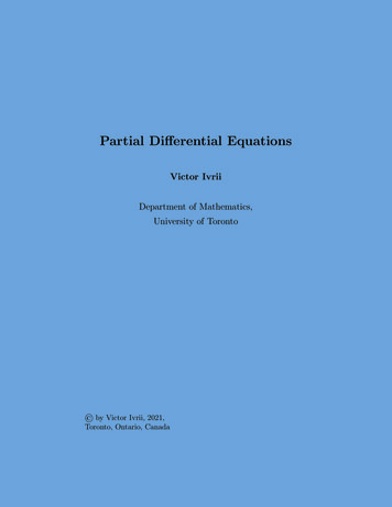
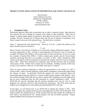
16J.D. Anderson, Jr.2.2 Modelling of the FlowIn obtaining the basic equations of fluid motion, the following philosophy is alwaysfollowed:(1) Choose the appropriate fundamental physical principles from the laws ofphysics, such as(a) Mass is conserved.(b) F ma (Newton’s 2nd Law).(c) Energy is conserved.(2) Apply these physical principles to a suitable model of the flow.(3) From this application, extract the mathematical equations which embody suchphysical principles.This section deals with item (2) above, namely the definition of a suitable model ofthe flow. This is not a trivial consideration. A solid body is rather easy to see anddefine; on the other hand, a fluid is a ‘squishy’ substance that is hard to grab holdof. If a solid body is in translational motion, the velocity of each part of the body isthe same; on the other hand, if a fluid is in motion the velocity may be different ateach location in the fluid. How then do we visualize a moving fluid so as to apply toit the fundamental physical principles?For a continuum fluid, the answer is to construct one of the two following models.2.2.1 Finite Control VolumeConsider a general flow field as represented by the streamlines in Fig. 2.1(a). Letus imagine a closed volume drawn within a finite region of the flow. This volumedefines a control volume, V, and a control surface, S, is defined as the closed surfacewhich bounds the volume. The control volume may be fixed in space with the fluidmoving through it, as shown at the left of Fig. 2.1(a). Alternatively, the controlvolume may be moving with the fluid such that the same fluid particles are alwaysinside it, as shown at the right of Fig. 2.1(a). In either case, the control volume is areasonably large, finite region of the flow. The fundamental physical principles areapplied to the fluid inside the control volume, and to the fluid crossing the controlsurface (if the control volume is fixed in space). Therefore, instead of looking atthe whole flow field at once, with the control volume model we limit our attentionto just the fluid in the finite region of the volume itself. The fluid flow equationsthat we directly obtain by applying the fundamental physical principles to a finitecontrol volume are in integral form. These integral forms of the governing equationscan be manipulated to indirectly obtain partial differential equations. The equationsso obtained from the finite control volume fixed in space (left side of Fig. 2.1a), ineither integral or partial differential form, are called the conservation form of thegoverning equations. The equations obtained from the finite control volume moving
2Governing Equations of Fluid Dynamics17Fig. 2.1 (a) Finite control volume approach. (b) Infinitesimal fluid element approachwith the fluid (right side of Fig. 2.1a), in either integral or partial differential form,are called the non-conservation form of the governing equations.2.2.2 Infinitesimal Fluid ElementConsider a general flow field as represented by the streamlines in Fig. 2.1b. Let usimagine an infinitesimally small fluid element in the flow, with a differential volume, dV. The fluid element is infinitesimal in the same sense as differential calculus; however, it is large enough to contain a huge number of molecules so that itcan be viewed as a continuous medium. The fluid element may be fixed in spacewith the fluid moving through it, as shown at the left of Fig. 2.1(b). Alternatively,it may be moving along a streamline with a vector velocity V equal to the flow velocity at each point. Again, instead of looking at the whole flow field at once, thefundamental physical principles are applied to just the fluid element itself. This application leads directly to the fundamental equations in partial differential equationform. Moreover, the particular partial differential equations obtained directly fromthe fluid element fixed in space (left side of Fig. 2.1b) are again the conservationform of the equations. The partial differential equations obtained directly from themoving fluid element (right side of Fig. 2.1b) are again called the non-conservationform of the equations.
18J.D. Anderson, Jr.In general aerodynamic theory, whether we deal with the conservation or nonconservation forms of the equations is irrelevant. Indeed, through simple manipulation,one form can be obtained from the other. However, there are cases in CFD where itis important which form we use. In fact, the nomenclature which is used to distinguish these two forms (conservation versus nonconservation) has arisen primarilyin the CFD literature.The comments made in this section become more clear after we have actuallyderived the governing equations. Therefore, when you finish this chapter, it wouldbe worthwhile to re-read this section.As a final comment, in actuality, the motion of a fluid is a ramification of the meanmotion of its atoms and molecules. Therefore, a third model of the flow can be amicroscopic approach wherein the fundamental laws of nature are applied directly tothe atoms and molecules, using suitable statistical averaging to define the resultingfluid properties. This approach is in the purview of kinetic theory, which is a veryelegant method with many advantages in the long run. However, it is beyond thescope of the present notes.2.3 The Substantial DerivativeBefore deriving the governing equations, we need to establish a notation which iscommon in aerodynamics—that of the substantial derivative. In addition, the substantial derivative has an important physical meaning which is sometimes not fullyappreciated by students of aerodynamics. A major purpose of this section is to emphasize this physical meaning.As the model of the flow, we will adopt the picture shown at the right ofFig. 2.1(b), namely that of an infinitesimally small fluid element moving with theflow. The motion of this fluid element is shown in more detail in Fig. 2.2. Here, thefluid element is moving through cartesian space. The unit vectors along the x, y, andz axes are i, j, and k respectively. The vector velocity field in this cartesian space isgiven by u i v j w kVwhere the x, y, and z components of velocity are given respectively byu u(x, y, z, t)v v(x, y, z, t)w w(x, y, z, t)Note that we are considering in general an unsteady flow, where u, v, and w arefunctions of both space and time, t. In addition, the scalar density field is given byρ ρ(x, y, z, t)
2Governing Equations of Fluid Dynamics19Fig. 2.2 Fluid elementmoving in the flowfield—illustration for thesubstantial derivativeAt time t1 , the fluid element is located at point 1 in Fig. 2.2. At this point andtime, the density of the fluid element isρ1 ρ(x1 , y1 , z1 , t1 )At a later time, t2 , the same fluid element has moved to point 2 in Fig. 2.2. Hence,at time t2 , the density of this same fluid element isρ2 ρ(x2 , y2 , z2 , t2 )Since ρ ρ(x, y, z, t), we can expand this function in a Taylor’s series about point1 as follows: ρ ρ ρρ2 ρ1 (x2 x1 ) (y2 y1 ) (z2 z1 ) x 1 y 1 z 1 ρ(t2 t1 ) (higher order terms) t 1Dividing by (t2 t1 ), and ignoring higher order terms, we obtain ρx2 x1 ρy2 y1ρ2 ρ1 t2 t1 x 1 t2 t1 yt2 t1 1 ρz2 z1 ρ z 1 t2 t1 t 1(2.1)Examine the left side of Eq. (2.1). This is physically the average time-rate-ofchange in density of the fluid element as it moves from point 1 to point 2. In thelimit, as t2 approaches t1 , this term becomes ρ2 ρ1Dρlim t2 t1 t2 t1Dt
20J.D. Anderson, Jr.Here, Dρ/Dt is a symbol for the instantaneous time rate of change of density ofthe fluid element as it moves through point 1. By definition, this symbol is called thesubstantial derivative, D/Dt. Note that Dρ/Dt is the time rate of change of densityof the given fluid element as it moves through space. Here, our eyes are locked on thefluid element as it is moving, and we are watching the density of the element changeas it moves through point 1. This is different from ( ρ/ t)1 , which is physically thetime rate of change of density at the fixed point 1. For ( ρ/ t)1 , we fix our eyeson the stationary point 1, and watch the density change due to transient fluctuationsin the flow field. Thus, Dρ/Dt and ρ/ρt are physically and numerically differentquantities.Returning to Eq. (2.1), note that x2 x1 ulimt2 t1 t2 t1 y2 y1lim vt2 t1 t2 t1 z2 z1lim wt2 t1 t2 t1Thus, taking the limit of Eq. (2.1) as t2 t1 , we obtainDρ ρ ρ ρ ρ u v w Dt x y z t(2.2)Examine Eq. (2.2) closely. From it, we can obtain an expression for the substantial derivative in cartesian coordinates:D u v wDt t x y z i j k x y zΔFurthermore, in cartesian coordinates, the vector operator(2.3)is defined as(2.4)ΔHence, Eq. (2.3) can be written asD V·Dt t(2.5)ΔEquation (2.5) represents a definition of the substantial derivative operator invector notation; thus, it is valid for any coordinate system.Focusing on Eq. (2.5), we once again emphasize that D/Dt is the substantialderivative, which is physically the time rate of change following a moving fluidelement; / t is called the local derivative, which is physically the time rate of · is called the convective derivative, which is physichange at a fixed point; Vcally the time rate of change due to the movement of the fluid element from oneΔ
2Governing Equations of Fluid Dynamics21location to another in the flow field where the flow properties are spatially different. The substantial derivative applies to any flow-field variable, for example,Dp/Dt, DT/Dt, Du/Dt, etc., where p and T are the static pressure and temperaturerespectively. For example: T · ) T T u T v T w T (V t t x y z convectivelocalderivativederivativeΔDT Dt(2.6)Again, Eq. (2.6) states physically that the temperature of the fluid element ischanging as the element sweeps past a point in the flow because at that point theflow field temperature itself may be fluctuating with time (the local derivative) andbecause the fluid element is simply on its way to another point in the flow fieldwhere the temperature is different (the convective derivative).Consider an example which will help to reinforce the physical meaning of thesubstantial derivative. Imagine that you are hiking in the mountains, and you areabout to enter a cave. The temperature inside the cave is cooler than outside. Thus,as you walk through the mouth of the cave, you feel a temperature decrease—thisis analagous to the convective derivative in Eq. (2.6). However, imagine that, atthe same time, a friend throws a snowball at you such that the snowball hits youjust at the same instant you pass through the mouth of the cave. You will feel anadditional, but momentary, temperature drop when the snowball hits you—this isanalagous to the local derivative in Eq. (2.6). The net temperature drop you feel asyou walk through the mouth of the cave is therefore a combination of both the actof moving into the cave, where it is cooler, and being struck by the snowball at thesame instant—this net temperature drop is analagous to the substantial derivative inEq. (2.6).The above derivation of the substantial derivative is essentially taken from thisauthor’s basic aerodynamics text book given as Ref. [1]. It is used there to introducenew aerodynamics students to the full physical meaning of the substantial derivative.The description is repeated here for the same reason—to give you a physical feel forthe substantial derivative. We could have circumvented most of the above discussionby recognizing that the substantial derivative is essentially the same as the totaldifferential from calculus. That is, ifρ ρ(x, y, z, t)then the chain rule from differential calculus gives ρ ρ ρ ρdx dy dz dt x y z t(2.7)dρ ρ ρ dx ρ dy ρ dz dt t x dt y dt z dt(2.8)dρ From Eq. (2.7), we have
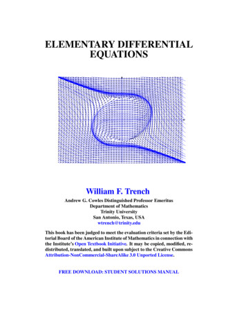
22SinceJ.D. Anderson, Jr.dydzdx u, v, and w, Eq. (2.8) becomesdtdtdtdρ ρ ρ ρ ρ u v wdt t x y z(2.9)Comparing Eqs. (2.2) and (2.9), we see that dρ/dt and Dρ/Dt are one-in-thesame.Therefore, the substantial derivative is nothing more than a total derivative withrespect to time. However, the derivation of Eq. (2.2) highlights more of the physicalsignificance of the substantial derivative, whereas the derivation of Eq. (2.9) is moreformal mathematically.Δ2.4 Physical Meaning of ·VAs one last item before deriving the governing equations, let us consider the diver This term appears frequently in the equations of fluidgence of the velocity, · V.dynamics, and it is well to consider its physical meaning.Consider a control volume moving with the fluid as sketched on the right ofFig. 2.1(a). This control volume is always made up of the same fluid particles as itmoves with the flow; hence, its mass is fixed, invariant with time. However, its volume V and control surface S are changing with time as it moves to different regionsof the flow where different values of ρ exist. That is, this moving control volumeof fixed mass is constantly increasing or decreasing its volume and is changing itsshape, depending on the characteristics of the flow. This control volume is shownin Fig. 2.3 at some instant in time. Consider an infinitesimal element of the surface as shown in Fig. 2.3. The change in the volumedS moving at the local velocity V,of the control volume ΔV , due to just the movement of dS over a time incrementΔt, is, from Fig. 2.3, equal to the volume of the long, thin cylinder with base area dS and altitude (VΔt)· n, where n is a unit vector perpendicular to the surface at dS .That is, ΔV (VΔt)· n dS (VΔt)· dS(2.10)Δwhere the vector dS is defined simply as dS n dS . Over the time increment Δt,the total change in volume of the whole control volume is equal to the summationof Eq. (2.10) over the total control surface. In the limit as dS 0, the sum becomesthe surface integralFig. 2.3 Moving controlvolume used for the physicalinterpretation of thedivergence of velocity
2Governing Equations of Fluid Dynamics23 (VΔt)· dSSIf this integral is divided by Δt, the result is physically the time rate of change ofthe control volume, denoted by DV/Dt, i.e. DV1 · dS (V · Δt) · dS V(2.11)DtΔtSSNote that we have written the left side of Eq. (2.11) as the substantial derivativeof V , because we are dealing with the time rate of change of the control volumeas the volume moves with the flow (we are using the picture shown at the right ofFig. 2.1a), and this is physically what is meant by the substantial derivative. Applying the divergence theorem from vector calculus to the right side of Eq. (2.11),we obtain DV ( · V)dV(2.12)DtVΔNow, let us image that the moving control volume in Fig. 2.3 is shrunk to a verysmall volume, δV , essentially becoming an infinitesimal moving fluid element assketched on the right of Fig. 2.1(a). Then Eq. (2.12) can be written as D(δV ) ( · V)dV(2.13)DtδVΔ is essentially the same valueAssume that δV is small enough such that · V .throughout δV . Then the integral in Eq. (2.13) can be approximated as ( · V)δVFrom Eq. (2.13), we haveΔΔD(δV ) ( · V)δVDtΔor ·V1 D(δV )δV Dt(2.14)ΔExamine Eq. (2.14) closely. On the left side we have the divergence of the velocity; on the right side we have its physical meaning. That is, is physically the time rate of change of the volume of a moving fluid element, per unit·Vvolume.Δ2.5 The Continuity EquationLet us now apply the philosophy discussed in Sect. 2.2; that is, (a) write down afundamental physical principle, (b) apply it to a suitable model of the flow, and(c) obtain an equation which represents the fundamental physical principle. In thissection we will treat the following case:
24J.D. Anderson, Jr.2.5.1 Physical Principle: Mass is ConservedWe will carry out the application of this principle to both the finite control volumeand infinitesimal fluid element models of the flow. This is done here specifically toillustrate the physical nature of both models. Moreover, we will choose the finitecontrol volume to be fixed in space (left side of Fig. 2.1a), whereas the infinitesimal fluid element will be moving with the flow (right side of Fig. 2.1b). In thisway we will be able to contrast the differences between the conservation and nonconservation forms of the equations, as described in Sect. 2.2.First, consider the model of a moving fluid element. The mass of this elementis fixed, and is given by δm. Denote the volume of this element by δV , as inSect. 2.4. Thenδm ρδV(2.15)Since mass is conserved, we can state that the time-rate-of-change of the massof the fluid element is zero as the element moves along with the flow. Invoking thephysical meaning of the substantial derivative discussed in Sect. 2.3, we haveD(δm) 0Dt(2.16)Combining Eqs. (2.15) and (2.16), we haveD(ρδV )DρD(δV ) δV ρ 0DtDtDtor,Dρ1 D(δV ) ρ 0DtδV Dt(2.17) We recognize the term in brackets in Eq. (2.17) as the physical meaning of · V,discussed in Sect. 2.4. Hence, combining Eqs. (2.14) and (2.17), we obtainΔDρ 0 ρ .VDt(2.18)ΔEquation (2.18) is the continuity equation in non-conservation form. In light of ourphilosophical discussion in Sect. 2.2, note that:(1) By applying the model of an infinitesimal fluid element, we have obtainedEq. (2.18) directly in partial differential form.(2) By choosing the model to be moving with the flow, we have obtained the nonconservation form of the continuity equation, namely Eq. (2.18).Now, consider the model of a finite control volume fixed in space, as sketched and the vectorin Fig. 2.4. At a point on the control surface, the flow velocity is Velemental surface area (as defined in Sect. 2.4) is dS . Also let dV be an elementalvolume inside the finite control volume. Applied to this control volume, our fundamental physical principle that mass is conserved means
2Governing Equations of Fluid Dynamics25Fig. 2.4 Finite controlvolume fixed in space Net mass flow out time rate of decrease ofcontrolvolumeofmassinsidecontrol through surface S volume (2.19a)B C(2.19b)or,where B and C are just convenient symbols for the left and right sides, respectively,of Eq. (2.19a). First, let us obtain an expression for B in terms of the quantitiesshown in Fig. 2.4. The mass flow of a moving fluid across any fixed surface (say, inkg/s, or slug/s) is equal to the product of (density) (area of surface) (componentof velocity perpendicular to the surface). Hence the elemental mass flow across thearea dS is · dS(2.20)ρVn dS ρVExamining Fig. 2.4, note that by convention, dS always points in a direction out also points out of the control volume (asof the control volume. Hence, when V · dS is positive. Moreover, when V points out ofshown in Fig. 2.4), the product ρVthe control volume, the mass flow is physically leaving the control volume, i.e. it is · dS denotes an outflow. In turn, when V points intoan outflow. Hence, a positive ρV the control volume, ρV · dS is negative. Moreover, when V points inward, the massflow is physically entering the control volume, i.e. it is an inflow. Hence, a negative · dS denotes an inflow. The net mass flow out of the entire control volume throughρVthe control surface S is the summation over S of the elemental mass flows shown inEq. (2.20). In the limit, this becomes a surface integral, which is physically the leftside of Eqs. (2.19a and b), i.e. · dSρV(2.21)B SNow consider the right side of Eqs. (2.19a and b). The mass contained within theelemental volume dV is ρ dV . The total mass inside the control volume is therefore ρ dVV
26J.D. Anderson, Jr.The time rate of increase of mass inside V is then ρ dV tVIn turn, the time rate of decrease of mass inside V is the negative of theabove, i.e. ρ dV C(2.22) tVThus, substituting Eqs. (2.21) and (2.22) into (2.19b), we have ρV · dS ρ dV tSVor, t V · dS 0ρVρ dV (2.23)SEquation (2.23) is the integral form of the continuity equation; it is also in conservation form.Let us cast Eq. (2.23) in the form of a differential equation. Since the controlvolume in Fig. 2.4 is fixed in space, the limits of integration for the integrals inEq. (2.23) are constant, and hence the time derivative / t can be placed inside theintegral. ρ · dS 0dV ρV(2.24)V tSApplying the divergence theorem from vector calculus, the surface integral inEq. (2.24) can be expressed as a volume integral · dS (ρV)· (ρV)dV(2.25)ΔVSSubstituting Eq. (2.25) into Eq. (2.24), we have ρ dV · (ρV)dV 0V tVΔorV ρ dV 0 · (ρV) tΔ (2.26)Since the finite control volume is arbitrarily drawn in space, the only way forthe integral in Eq. (2.26) to equal zero is for the integrand to be zero at every pointwithin the control volume. Hence, from Eq. (2.26) ρ 0 · (ρV) t(2.27)Δ
2Governing Equations of Fluid Dynamics27Equation (2.27) is the continuity equation in conservation form.Examining the above derivation in light of our discussion in Sect. 2.2, wenote that:(1) By applying the model of a finite control volume, we have obtained Eq. (2.23)directly in integral form.(2) Only after some manipulation of the integral form did we indirectly obtain apartial differential equation, Eq. (2.27).(3) By choosing the model to be fixed in space, we have obtained the conservationform of the continuity equation, Eqs. (2.23) and (2.27).Emphasis is made that Eqs. (2.18) and (2.27) are both statements of the conservation of mass expressed in the form of partial differential equations. Eq. (2.18) isin non-conservation form, and Eq. (2.27) is in conservation form; both forms areequally valid. Indeed, one can easily be obtained from the other, as follows. Consider the vector identity involving the divergence of the product of a scalar times avector, such as ρ ·V V · ρ· (ρV)(2.28)ΔΔΔSubstitute Eq. (2.28) in the conservation form, Eq. (2.27): ρ 0 V · ρ ρ ·V t(2.29)ΔΔThe first two terms on the left side of Eq. (2.29) are simply the substantial derivative of density. Hence, Eq. (2.29) becomesDρ 0 ρ ·VDtΔwhich is the non-conservation form given by Eq. (2.18).Once again we note that the use of conservation or non-conservation forms ofthe governing equations makes little difference in most of theoretical aerodynamics.In contrast, which form is used can make a difference in some CFD applications,and this is why we are making a distinction between these two different forms in thepresent notes.2.6 The Momentum EquationIn this section, we apply another fundamental physical principle to a model of theflow, namely:Physical Principle :F m a (Newton’s 2nd law)We choose for our flow model the moving fluid element as shown at the right ofFig. 2.1(b). This model is sketched in more detail in Fig. 2.5.Newton’s 2nd law, expressed above, when applied to the moving fluid elementin Fig. 2.5, says that the net force on the fluid element equals its mass times the
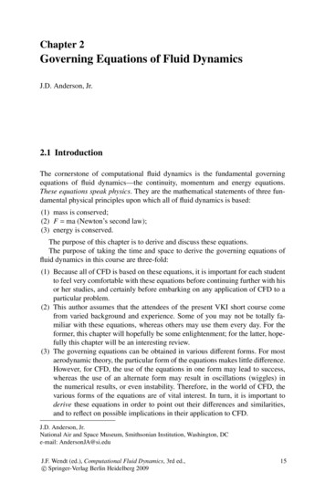
28J.D. Anderson, Jr.Fig. 2.5 Infinitesimally small, moving fluid element. Only the forces in the x direction are shownacceleration of the element. This is a vector relation, and hence can be split into threescalar relations along the x, y, and z-axes. Let us consider only the x-component ofNewton’s 2nd law,(2.30)Fx maxwhere Fx and ax are the scalar x-components of the force and accelerationrespectively.First, consider the left side of Eq. (2.30). We say that the moving fluid elementexperiences a force in the x-direction. What is the source of this force? There aretwo sources:(1) Body forces, which act directly on the volumetric mass of the fluid element.These forces ‘act at a distance’; examples are gravitational, electric and magnetic forces.(2) Surface forces, which act directly on the surface of the fluid element. They aredue to only two sources: (a) the pressure distribution acting on the surface, imposed by the outside fluid surrounding the fluid element, and (b) the shear andnormal stress distributions acting on the surface, also imposed by the outsidefluid ‘tugging’ or ‘pushing’ on the surface by means of friction.Let us denote the body force per unit mass acting on the fluid element by f , withfx as its x-component. The volume of the fluid element is (dx dy dz); hence, Body force on the fluidelementacting ρ fx (dx dy dz) in the x-direction (2.31)
2Governing Equations of Fluid Dynamics29Fig. 2.6 Illustration of shear and normal stressesThe shear and normal stresses in a fluid are related to the time-rate-of-change ofthe deformation of the fluid element, as sketched in Fig. 2.6 for just the xy plane.The shear stress, denoted by τxy in this figure, is related to the time rate-of-change ofthe shearing deformation of the fluid element, whereas the normal stress, denoted byτxx in Fig. 2.6, is related to the time-rate-of-change of volume of the fluid element.As a result, both shear and normal stresses depend on velocity gradients in the flow,to be designated later. In most viscous flows, normal stresses (such as τxx ) are muchsmaller than shear stresses, and many times are neglected. Normal stresses (sayτxx in the x-direction) become important when the normal velocity gradients (say u/ x) are very large, such as inside a shock wave.The surface forces in the x-direction exerted on the fluid element are sketchedin Fig. 2.5. The convention will be used here that τij denotes a stress in thej-direction exerted on a plane perpendicular to the i-axis. On face abcd, the onlyforce in the x-direction is that due to shear stress, τyx dx dz. Face efgh is a distance dy above face abcd; hence the shear force in the x-direction on face efgh is[τyx ( τyx / y) dy] dx dz. Note the directions of the shear force on faces abcdand efgh; on the bottom face, τyx is to the left (the negative x-direction), whereason the top face, [τyx ( τyx / y) dy] is to the right (the positive x-direction).These directions are consistent with the convention that positive increases in allthree components of velocity. u, v and w, occur in the positive directions of theaxes. For example, in Fig. 2.5, u increases in the positive y-direction. Therefore, concentrating on face efgh, u is higher just above the face than on theface; this causes a ‘tugging’ action which tries to pull the fluid element in thepositive x-direction (to the right) as shown in Fig. 2.5. In turn, concentratingon face abcd, u is lower just beneath the face than on the face; this causes aretarding or dragging action on the fluid element, which acts in the negativex-direction (to the left) as shown in Fig. 2.5. The directions of all the other viscous stresses shown in Fig. 2.5, including τxx , can be justified in a like fashion.Specifically on face dcgh, τzx acts in the negative x-direction, whereas on face abfe,[τzx ( τzx / z) dz] acts in the positive x-direction. On face adhe, which is perpendicular to the x-axis, the only forces in the x-direction are the pressure forcep dx dz, which always acts in the direction into the fluid element, and τxx dy dz,which is in the negative x-direction. In Fig. 2.5, the reason why τxx on face adhe isto the left hinges on the convention mentioned earlier for the direction of increasing
30J.D. Anderson, Jr.velocity. Here, by convention, a positive increase in u takes place in the positivex-direction. Hence, the value of u just to the left of face adhe is smaller than thevalue of u on the face itself. As a result, the viscous action of the normal stressacts as a ‘suction’ on face adhe, i.e. there is a dragging action toward the left thatwants to retard the motion of the fluid element. In contrast, on face bcgf, the pressure force [p ( p/ x) dx] dy dz presses inward on the fluid element (in the negativex-direction), and because the value of u just to the right of face bcgf is larger thanthe value of u on the face, there is a ‘suction’ due to the viscous normal stress whichtries to pul
20 J.D. Anderson, Jr. Here, Dρ/Dt is a symbol for the instantaneous time rate of change of density of the fluid element as it moves through point 1. By definition, this symbol is called the substantial derivative, D/Dt.Note that Dρ/Dt is the time rate of change of density of the given fluid element as