Transcription
PROJECTS WITH APPLICATIONS OF DIFFERENTIAL EQUATIONS AND MATLABDavid SzurleyFrancis Marion UniversityDepartment of MathematicsPO Box 100547Florence, SC l equations (DEs) play a prominent role in today’s industrial setting. Many physicallaws describe the rate of change of a quantity with respect to other quantities. Since “rate ofchange” is simply another phrase for derivative, these physical laws may be written as DEs. Forexample, Newton’s Second Law of Motion states that the rate of change of momentum of anobject is equal to the sum of the imposed forces. Normally this is written asF mam ,where F represents the total imposed force. However, if we let x denote the position of theobject, then this may be rewritten asF m&x&.Hence, Newton’s Second Law of Motion is a second-order ordinary differential equation. Thereare many applications of DEs. Growth of microorganisms and Newton’s Law of Cooling areexamples of ordinary DEs (ODEs), while conservation of mass and the flow of air over a wingare examples of partial DEs (PDEs). Further, predator-prey models and the Navier-Stokesequations governing fluid flow are examples of systems of DEs. Many introductory ODEcourses are devoted to solution techniques to determine the analytic solution of a given, normallylinear, ODE. While these techniques are important, many real-life processes may be modeledwith systems of DEs. Further, these systems may be nonlinear. Nonlinear systems of DEs maynot have exact solutions. However, we still desire some type of “solution”.There are many numerical techniques to obtain an approximation to the solution of a DE orsystem of DEs. Many scientific packages contain library commands to numerically approximatethe solution of these. In particular, MATLAB contains the ode45 command which willnumerically approximate the solution to a system of ODEs using a medium order method. Thus,the scientific package MATLAB may be used to explore DEs modeling real-world applicationsthat are more complicated than the DEs presented in a typical introductory course. UsingMATLAB also has the advantage that the internal command guide may be used to creategraphical user interfaces (GUIs) to help facilitate this exploration. The GUIs ensure that thestudents are not bogged down with reading and understanding MATLAB code.In this paper, we will discuss how to use MATLAB to simulate the solution to DEs. Thenprojects the author has assigned involving real-world applications of DEs will be described. Oneproject models the industrial process of film casting while the other models the conduction ofheat within a one-dimensional rod. Similar projects will also be briefly described. Finally,student feedback from the projects will be given.234
II.SIMULATING SOLUTIONS TO ORDINARY DIFFERENTIAL EQUATIONS INMATLABMATLAB provides many commands to approximate the solution to DEs: ode45, ode15s, andode23 are three examples. Suppose that the system of ODEs is written in the formy' f t , y ,where y represents the vector of dependent variables and f represents the vector of right-handside functions. All of the commands (e.g., ode45) require three arguments:a filename which returns the value of the right-hand-side vector f ,vector representing the domain of the independent variable t ,set of initial conditions.Consider the DE that models driven, damped spring motion.2&x& 2 x&x FFigure 1 contains a portion of the MATLAB code used to numerically approximate the solutionto this DE.Figure 1: MATLAB code.Some notes are in order here.The internal commands ode45, ode15s, etc. only accept first-order DEs.Many higher-order DEs may be transformed into systems of first-order DEs.The order of the formal arguments in SpringMass is important.T represents the values of the independent variable t generated by ode45.Each row in X represents the value of X corresponding to the associated time value in T.Once the solution is obtained, the output may be displayed via the internal command plot; frillsmay be added as needed. Figure 2 contains the portion of code used to display theapproximation.235
Figure 2: MATLAB code used to produce the display of the approximation.The natural next step is to provide students with this code and ask questions. For example, onecould ask students what is the effect of changing the damping coefficient. In order for thestudents to answer this question, they are required to determine the line(s) in the code where thedamping coefficient is defined, appropriately change those, and rerun the code. This processdemonstrates a drawback to using this approach: it is difficult for the students to read andunderstand code.One solution to this problem is the use of GUIs. They provide a means of introducing studentsto scientific packages without entirely involving the students within the code. Instead ofexpecting students to modify code, they may simply edit text and click a button. The requiredcalculations are then accomplished for the students without being visible. The MATLABinternal command guide is the GUI development interface. It enables simplified arrangementand sizing of GUI components as well as auto-generation of code for these components.Examples of GUI components would be push buttons, axes, sliders, pop-up menus, amongothers. Figure 3 displays an example GUI for the spring-mass system.Figure 3: Example GUI for the spring-mass system.236
The students may change the quantities by simply typing the new value in the edit text boxes andrerun the code by pressing the push button. With this GUI, it is easier for students to answerquestions related to changing system parameters. Now the students may explore the particularmodel by being provided with the GUI and some auxiliary files.III. PROJECTSStudents enrolled in an introductory ordinary differential equations course were grouped up andgiven different projects. Each project involved an industrial process that may be modeled byDEs. The students were asked to understand the process, why it is useful, how the process ismodeled, and to present their results at a conference. There were four main thrusts of theprojects.Expose students to a real-world processExpose students to a scientific software package (MATLAB)Demonstrate the need for numerical schemesGain experience in public speaking via presentation of their resultsIV. FILM CASTINGToday’s society has in great abundance products that are made from polymers: clothing madefrom synthetic fibers, plastic bags, food wrap, and disposable diapers are among the mostcommon examples. It has become imperative for today’s manufacturers to understand theprocesses used to make these products as fully as possible. The processes involve complex fluidflow of a molten polymer, governed by systems of DEs.Film casting is an industrial process in which fluid (molten polymer) is extruded from arectangular die of thickness e 0 and length l 0 , at a temperature T0 , and a velocity u 0 . Please see[1], [3], [6], [9] – [12], and [13] for a detailed description of the process. The fluid is thenstretched in the air due to the constant pulling force F of the chill roll, located at a distance of Lfrom the die. The film is then cooled on this chill roll to solidify the fluid. The film castingprocess is shown in Figure 4.Figure 4: Schematic of the film casting process.237
The five dependent variables of the flow are length l , velocity u , pulling force F , temperatureT , and thickness e . Under certain assumptions, the equations governing this process may bedldx12 ududx1242 362lF8A2u22F 2Al2FAdFdxl2dT2hTC p uedxgiven as follows.TT4T4dedxdudxAgAd edxdl edx lAuAdu edx uThis is a system of five first order nonlinear ODEs. Further, while the initial conditions forlength, velocity, temperature, and thickness are simply those at the die exit, the initial pullingforce F0 is not known a priori. The numerical technique of shooting is used to determine thevalue of F0 . As opposed to attempting to solve this system analytically, it would be better tonumerically approximate the solution using a numerical package (e.g., ode45).Code was written that will numerically simulate the solution to these equations given a set ofparameters. Moreover, a GUI was designed so that students were required to only edit theparameters. Figure 5 displays the GUI provided to the students as well as a typical solutionprofile. Students were asked to change the set of parameters and to determine the effect thechange had on the solution.Figure 5: GUI and typical solution profile for the film casting problem.238
V.HEAT CONDUCTION IN A ONE-DIMENSIONAL RODThe manner in which heat is transferred within a one-dimensional rod may be modeled with aPDE. We assume an initial temperature distribution and desire to know how heat is conductedwithin the rod as time evolves. The PDE that models heat conduction may be given by2uuk 2,txwhere k is the thermal diffusivity (see [8]). We assume that the initial temperature distributionis prescribed and that the temperature at the ends of the rod ( x 0 and x L ) are given. Hencethe boundary and initial conditions areu (0, t ) 0,u ( L, t )u ( x, 0)0,f ( x).Since this is a PDE, the suite of ODE solvers in MATLAB are inappropriate. Hence, we chooseto numerically approximate the solution to this PDE via the finite difference method (FDM). See[8] for a rough description of the FDM. The FDM first takes the continuous domain in the xt plane and replaces it with a discrete mesh, as shown in Figure 6.Figure 6: Example of a FDM mesh.Next, the partial derivatives in the PDE itself are replaced with approximately equivalentudifference quotients. If we let u (jm ) u ( x j , t m ) , choose to approximatewith a forwardt2udifference andwith a centered difference, we obtain the following finite differencet2equation.k tu (jm 1) u (jm )u (jm1) 2u (jm ) u (jm1)2x239
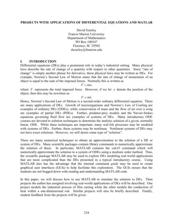
Code was written to solve the finite difference equation and display the results. Once the codewas working properly, a GUI was designed to allow students to numerically approximate thesolution for a given parameter set. Figure 7 shows the GUI as well as a solution profile for aparameter set.Figure 7: GUI and solution profile for heat conduction in a one-dimensional rod.Students were asked to change the initial condition and the thermal diffusivity to determine theeffect on the solution profile.VI. FIBER SPINNING PROJECTSTwo projects involved the industrial process of fiber spinning (see [2], [4], [5], [7], and [14]). Inthis process, an axisymmetric stream of polymer melt is extruded from a spinneret containingthousands of capillaries. The spinneret may be thought of roughly as a shower head. Thepolymer melt is then drawn continuously by the take-up rolls. Along the length of the stream,there is a region where cooling air is applied. This process is illustrated in Figure 8.240
Figure 8: Schematic of the fiber spinning process.Depending upon the processing parameters, the polymer may enter a semi-crystalline phasewhere the structure of the molecules of the polymer cannot change. One project explored fiberspinning excluding the semi-crystalline phase, while the other project considered both phases.Both processes are governed by systems of nonlinear ordinary differential equations.VII. WAVE PROPAGATION PROJECTThe final project explored the propagation of waves on a taut string (see [8]). This process isgoverned by the following PDE.22uu2c2tx2Here c represents the propagation speed of the wave. The following boundary and initialconditions are enforced.u (0, t ) 0u ( L, t ) 0u ( x, 0) f ( x)u( x, 0) g ( x)tFigure 9 displays the GUI provided to the students as well as an example solution profile.\241
Figure 9: GUI and solution profile for wave propagation on a taut string.Students were asked to change the initial displacement of the string and the propagation speed todetermine the effect on the solution profile.VIII. STUDENT FEEDBACKStudent response from these projects differed between the objectives of the projects. Studentresponses were generally positive about exploring real-world applications of DEs and theexperience gained in public speaking. However, the responses were generally mediocre for thenumerical schemes and the exposure to MATLAB. Many students were surprised that DEsmodeling real-world applications could not be solved analytically. Overall, the students gave theprojects positive reviews and considered them a success.REFERENCES[1] Acierno, D., L. Di Maio, C. Ammirati, “Film Casting of Polyethylene Terephthalate:Experiments and Model Comparisons,” Polymer Engineering and Science, Vol. 40, pp. 108117, 2000.[2] Advani, S., C. Tucker III, “The Use of Tensors to Describe and Predict Fiber Orientation InShort Fiber Composites,” Journal of Rheology, Vol. 31, pp. 751-784, 1987.[3] Baird, D., D. Collais, Polymer Processing, John Wiley and Sons, New York, 1998.[4] Denn, M., Process Modeling, Longman Inc., New York, 1986.[5] Doufas, A., A, McHugh, C. Miller, “Simulation of Melt Spinning Including Flow-InducedCrystallization Part I: Model Development and Predictions,” Journal of Non-NewtonianFluid Mechanics, Vol. 92, pp. 27-66, 2000.[6] Eisele, P., R. Killpack, “Propene,” Ullman’s Encyclopedia of Industrial Chemistry, 1993 ed.[7] Fisher, R., M. Denn, “Mechanics of Nonisothermal Polymer Melt Spinning,” AmericanInstitute of Chemical Engineers Journal, Vol. 23, No. 1, pp. 23-28.[8] Haberman, R., Elementary Applied Partial Differential Equations, Prentice Hall, New Jersey,1987.[9] Lide, D., ed. CRC Handbook of Chemistry and Physics, CRC Press, New York, 2001.[10] Mark, J., ed. Physical Properties of Polymers Handbook, AIP Press New York 1996.242
[11][12][13][14]Smith, S., D. Stolle, “Nonisothermal Two-Dimensional Film Casting of a ViscousPolymer,” Polymer Engineering and Science, Vol. 40, pp. 1870-1877, 2000.Vargaftik, N., Tables on the Thermophysical Properties of Liquids and Gases, JohnWiley and Sons, New York, 1
are examples of partial DEs (PDEs). Further, predator-prey models and the Navier-Stokes equations governing fluid flow are examples of systems of DEs. Many introductory ODE courses are devoted to solution techniques to determine the analytic solution of a given, normally linear, ODE. While these techniques are important, many real-life .