WIXLIB

Chapter 1Introduction1.1PDE motivations and contextThe aim of this is to introduce and motivate partial differential equations(PDE). The section also places the scope of studies in APM346 within thevast universe of mathematics. A partial differential equation (PDE) is angather involving partial derivatives. This is not so informative so let’s breakit down a bit.1.1.1What is a differential equation?An ordinary differential equation (ODE) is an equation for a function whichdepends on one independent variable which involves the independent variable,the function, and derivatives of the function:F (t, u(t), u0 (t), u(2) (t), u(3) (t), . . . , u(m) (t)) 0.This is an example of an ODE of order m where m is a highest order ofthe derivative in the equation. Solving an equation like this on an intervalt [0, T ] would mean finding a function t 7 u(t) R with the propertythat u and its derivatives satisfy this equation for all values t [0, T ].The problem can be enlarged by replacing the real-valued u by a vectorvalued one u(t) (u1 (t), u2 (t), . . . , uN (t)). In this case we usually talkabout system of ODEs.Even in this situation, the challenge is to find functions dependingupon exactly one variable which, together with their derivatives, satisfy theequation.1

Chapter 1. Introduction2What is a partial derivative?When you have function that depends upon several variables, you candifferentiate with respect to either variable while holding the other variableconstant. This spawns the idea of partial derivatives. As an example,consider a function depending upon two real variables taking values in thereals:u : Rn R.As n 2 we sometimes visualize a function like this by considering itsgraph viewed as a surface in R3 given by the collection of points{(x, y, z) R3 : z u(x, y)}.We can calculate the derivative with respect to x while holding y fixed. This leads to ux , also expressed as x u, u, and xu. Similarly, we can hold xx fixed and differentiate with respect to y.What is PDE?A partial differential equation is an equation for a function which dependson more than one independent variable which involves the independentvariables, the function, and partial derivatives of the function:F (x, y, u(x, y), ux (x, y), uy (x, y), uxx (x, y), uxy (x, y), uyx (x, y), uyy (x, y)) 0.This is an example of a PDE of order 2. Solving an equation like thiswould mean finding a function (x, y) u(x, y) with the property that uand its derivatives satisfy this equation for all admissible arguments.Similarly to ODE case this problem can be enlarged by replacing thereal-valued u by a vector-valued one u(t) (u1 (x, y), u2 (x, y), . . . , uN (x, y).In this case we usually talk about system of PDEs.Where PDEs are coming from?PDEs are often referred as Equations of Mathematical Physics (or Mathematical Physics but it is incorrect as Mathematical Physics is now a separatefield of mathematics) because many of PDEs are coming from different

Chapter 1. Introduction3domains of physics (acoustics, optics, elasticity, hydro and aerodynamics,electromagnetism, quantum mechanics, seismology etc).However PDEs appear in other fields of science as well (like quantumchemistry, chemical kinetics); some PDEs are coming from economics andfinancial mathematics, or computer science.Many PDEs are originated in other fields of mathematics.Examples of PDEs(Some are actually systems)Simplest first order equationux 0.Transport equationut cux 0. equation : 1 (fx ify ) 0, f2( is known as “di-bar” or Wirtinger derivatives), or as f u iv(ux vy 0,uy vx 0.Those who took Complex variables know that those are Cauchy-Riemannequations.Laplace’s equation (in 2D) u : uxx uyy 0or similarly in the higher dimensions.

Chapter 1. Introduction4Heat equationut k u;(The expression is called the Laplacian (Laplace operator ) and is definedas x2 y2 z2 on R3 ).Schrödinger equation (quantum mechanics) 2 V ψ.2mHere ψ is a complex-valued function.i t ψ Wave equationutt c2 u 0;sometimes : c 2 t2 is called (d’Alembertian or d’Alembert operator ).It appears in elasticity, acoustics, electromagnetism and so on.One-dimensional wave equationutt c2 uxx 0often is called string equation and describes f.e. a vibrating string.Oscillating rod or plate (elasticity) Equation of vibrating rod (withone spatial variable)utt Kuxxxx 0or vibrating plate (with two spatial variables)utt K 2 u 0.Maxwell equations (electromagnetism) in vacuum E t c H 0,H t c E 0, · E · H 0.Here E and H are vectors of electric and magnetic intensities, so the firsttwo lines are actually 6 6 system. The third line means two more equations,and we have 8 6 system. Such systems are called overdetermined.

Chapter 1. Introduction5Dirac equations (relativistic quantum mechanics)X i t ψ βmc2 ic αk xk ψ1 k 3with Dirac 4 4-matrices α1 , α2 , α3 , β. Here ψ is a complex 4-vector, so infact we have 4 4 system.Elasticity equations (homogeneous and isotropic)utt λ u µ ( · u).homogeneous means “the same in all places” (an opposite is calledinhomogeneous) and isotropic means “the same in all directions” (an oppositeis called anisotropic).Navier-Stokes equation (hydrodynamics for incompressible liquid)(ρv t (v · )ρv ν v p, · v 0,where ρ is a (constant) density, v is a velocity and p is the pressure; whenviscosity ν 0 we get Euler equation(ρv t (v · )ρv p, · v 0.Both of them are 4 4 systems.Yang-Mills equation (elementary particles theory) xj Fjk [Aj , Fjk ] 0,Fjk : xj Ak xk Aj [Aj , Ak ],where Ak are traceless skew-Hermitian matrices. Their matrix elements areunknown functions. This is a 2nd order system.

Chapter 1. Introduction6Einstein equation for general relativityGµν Λgµν κTµν ,where Gµν Rµν 12 gµν is the Einstein tensor, gµν is the metric tensor(unknown functions), Rµν is the Ricci curvature tensor, and R is the scalarcurvature, Tµν is the stress–energy tensor, Λ is the cosmological constantand κ is the Einstein gravitational constant. Components of Ricci curvaturetensor are expressed through the components of the metric tensor, their firstand second derivatives. This is a 2nd order system.Black-Scholes equation Black-Scholes Equation (Financial mathematics)is a partial differential equation (PDE) governing the price evolution of aEuropean call or European put under the Black–Scholes model. Broadlyspeaking, the term may refer to a similar PDE that can be derived for avariety of options, or more generally, derivatives: V1 V 2V σ 2 S 2 2 rS rV 0 t2 S Swhere V is the price of the option as a function of stock price S and time t,r is the risk-free interest rate, and σ is the volatility of the stock.Do not ask me what this means!Remark 1.1.1. (a) Some of these examples are actually not single PDEs butthe systems of PDEs.(b) In all this examples there are spatial variables x, y, z and often timevariable t but it is not necessarily so in all PDEs. Equations, not includingtime, are called stationary (an opposite is called nonstationary).(c) Equations could be of different order with respect to different variablesand it is important. However if not specified the order of equation is thehighest order of the derivatives invoked.(d) In this class we will deal mainly with the wave equation, heat equationand Laplace equation in their simplest forms.

Chapter 1. Introduction1.21.2.17Initial and boundary value problemsProblems for PDEsWe know that solutions of ODEs typically depend on one or several constants.For PDEs situation is more complicated. Consider simplest equationsux 0,vxx 0wxy 0(1.2.1)(1.2.2)(1.2.3)with u u(x, y), v v(x, y) and w w(x, y). Equation (1.2.1) could betreaded as an ODE with respect to x and its solution is a constant but thisis not a genuine constant as it is constant only with respect to x and candepend on other variables; so u(x, y) φ(y).Meanwhile, for solution of (1.2.2) we have vx φ(y) where φ is anarbitrary function of one variable and it could be considered as ODE withrespect to x again; then v(x, y) φ(y)x ψ(y) where ψ(y) is anotherarbitrary function of one variable.Finally, for solution of (1.2.3) we have wy φ(y) where φ is an arbitraryfunction of one variable and it could beR considered as ODE with respect toy; then (w g(y))y 0 where g(y) φ(y) dy, and therefore w g(y) f (x) w(x, y) f (x) g(y) where f, g are arbitrary functions of onevariable.Considering these equations again but assuming that u u(x, y, z),v v(x, y, z) we arrive to u φ(y, z), v φ(y, z)x ψ(y, z) and w f (x, z) g(y, z) where f, g are arbitrary functions of two variables.Solutions to PDEs typically depend not on several arbitrary constantsbut on one or several arbitrary functions of n 1 variables. For morecomplicated equations this dependence could be much more complicated andimplicit. To select a right solutions we need to use some extra conditions.The sets of such conditions are called Problems. Typical problems are(a) IVP (Initial Value Problem): one of variables is interpreted as time tand conditions are imposed at some moment; f.e. u t t0 u0 ;(b) BVP (Boundary Value Problem) conditions are imposed on the boundary of the spatial domain Ω: f.e. u Ω φ where Ω is a boundary ofΩ and φ is defined on Ω;

Chapter 1. Introduction8(c) IVBP (Initial-Boundary Value Problem a.k.a. mixed problem): one ofvariables is interpreted as time t and some conditions are imposed atsome moment but other conditions are imposed on the boundary ofthe spatial domain.Remark 1.2.1. In the course of ODEs students usually consider IVP only.F.e. for the second-order equation likeuxx a1 ux a2 u f (x)such problem is u x x0 u0 , ux x x0 u1 . However one could considerBVPs like(α1 ux β1 u) x x1 φ1 ,(α2 ux β2 u) x x2 φ2 ,where solutions are sought on the interval [x1 , x2 ]. Such are covered inadvanced chapters of some of ODE textbooks (but not covered by a typicalODE class). We will need to cover such problems later in this class.1.2.2Notion of “well-posedness”We want that our PDE (or the system of PDEs) together with all theseconditions satisfied the following requirements:(a) Solutions must exist for all right-hand expressions (in equations andconditions)–existence;(b) Solution must be unique–uniqueness;(c) Solution must depend on these right-hand expressions continuously,which means that small changes in the right-hand expressions lead tosmall changes in the solution.Such problems are called well-posed. PDEs are usually studied togetherwith the problems which are well-posed for these PDEs. Different types ofPDEs admit different problems.Sometimes however one needs to consider ill-posed problems. In particular, inverse problems of PDEs are almost always ill-posed.

Chapter 1. Introduction1.31.3.19Classification of equationsLinear and nonlinear equationsEquations of the formLu f (x)(1.3.1)where Lu is a partial differential expression linear with respect to unknownfunction u is called linear equation (or linear system). This equation islinear homogeneous equation if f 0 and linear inhomogeneous equationotherwise. For example,Lu : a11 uxx 2a12 uxy a22 uyy a1 ux a2 uy au f (x)(1.3.2)is linear; if all coefficients ajk , aj , a are constant, we call it linear equationwith constant coefficients; otherwise we talk about variable coefficients.Otherwise equation is called nonlinear. However there is a more subtleclassification of such equations. Equations of the type (1.3.1), where the righthand expression f depends on the solution and its lower-order derivatives,are called semilinear, equations where both coefficients and right-handexpression depend on the solution and its lower-order derivatives are calledquasilinear. For example,Lu : a11 (x, y)uxx 2a12 (x, y)uxy a22 (x, y)uyy f (x, y, u, ux , uy )(1.3.3)is semilinear, andLu : a11 (x, y, u, ux , uy )uxx 2a12 (x, y, u, ux , uy )uxy a22 (x, y, u, ux , uy )uyy f (x, y, u, ux , uy ) (1.3.4)is quasilinear, whileF (x, y, u, ux , uy , uxx , uxy , uyx ) 0(1.3.5)is general nonlinear.1.3.2Elliptic, hyperbolic and parabolic equationsGeneral Consider second order equation (1.3.2):XLu : aij uxi xj l.o.t. f (x)1 i,j n(1.3.6)

Chapter 1. Introduction10where l.o.t. means lower order terms (that is, terms with u and its lowerorder derivatives) with aij aji . Let us change variables x x(x0 ). Thenthe matrix of principal coefficients a11 . . . a1n . . . . . A an1 . . . annin the new coordinate system becomes A0 Q AQ where Q T 1 and xiT xis a Jacobi matrix. The proof easily follows from the0ji,j 1,.,nchain rule (Calculus II).Therefore if the principal coefficients are real and constant, by a linearchange of variables matrix of the principal coefficients could be reducedto the diagonal form, where diagonal elements could be either 1, or 1 or0. Multiplying equation by 1 if needed we can assume that there are atleast as many 1 as 1. In particular, for n 2 the principal part becomeseither uxx uyy , or uxx uyy , or uxx and such equations are called elliptic,hyperbolic, and parabolic respectively (there will be always second derivativesince otherwise it would be the first order equation).This terminology comes from the curves of the second order conicalsections: if a11 a22 a212 0 equationa11 ξ 2 2a12 ξη a22 η 2 a1 ξ a2 η cgenerically defines an ellipse, if a11 a22 a212 0 this equation genericallydefines a hyperbole and if a11 a22 a212 0 it defines a parabole.Let us consider equations in different dimensions:2D If we consider only 2-nd order equations with constant real coefficientsthen in appropriate coordinates they will look like eitheruxx uyy l.o.t f(1.3.7)uxx uyy l.o.t. f,(1.3.8)orwhere l.o.t. mean lower order terms, and we call such equations elliptic andhyperbolic respectively.

Chapter 1. Introduction11What to do if one of the 2-nd derivatives is missing? We get parabolicequationsuxx cuy l.o.t. f.(1.3.9)with c 6 0 (we do not consider cuy as a lower order term here) and IVPu y 0 g is well-posed in the direction of y 0 if c 0 and in directiony 0 if c 0. We can dismiss c 0 as not-interesting.However this classification leaves out very important Schrödinger equationuxx icuy 0(1.3.10)with real c 6 0. For it IVP u y 0 g is well-posed in both directions y 0 andy 0 but it lacks many properties of parabolic equations (like maximumprinciple or mollification; still it has interesting properties on its own).3D Again, if we consider only 2-nd order equations with constant realcoefficients, then in appropriate coordinates they will look like eitheruxx uyy uzz l.o.t f(1.3.11)uxx uyy uzz l.o.t. f,(1.3.12)orand we call such equations elliptic and hyperbolic respectively.Also we get parabolic equations likeuxx uyy cuz l.o.t. f.(1.3.13)uxx uyy cuz l.o.t. f ?(1.3.14)What aboutAlgebraist-formalist would call it parabolic-hyperbolic but since this equationexhibits no interesting analytic properties (unless one considers lack of suchproperties interesting; in particular, IVP is ill-posed in both directions) itwould be a perversion.Yes, there will be Schrödinger equationuxx uyy icuz 0(1.3.15)with real c 6 0 but uxx uyy icuz 0 would also have IVP u z 0 gwell-posed in both directions.

Chapter 1. Introduction124D Here we would get also ellipticuxx uyy uzz utt l.o.t. f,(1.3.16)uxx uyy uzz utt l.o.t. f,but also ultrahyperbolicuxx uyy uzz utt l.o.t. f,(1.3.17)hyperbolic(1.3.18)which exhibits some interesting analytic properties but these equations areway less important than elliptic, hyperbolic or parabolic.Parabolic and Schrödinger will be here as well.Remark 1.3.1. (a) The notions of elliptic, hyperbolic or parabolic equationsare generalized to higher dimensions (trivially) and to higher-order equations,but most of the randomly written equations do not belong to any of thesetypes and there is no reason to classify them.(b) There is no complete classifications of PDEs and cannot be because anyreasonable classification should not be based on how equation looks like buton the reasonable analytic properties it exhibits (which IVP or BVP arewell-posed etc).Equations of the variable type To make things even more complicatedthere are equations changing types from point to point, f.e. Tricomi equationuxx xuyy 0(1.3.19)which is elliptic as x 0 and hyperbolic as x 0 and at x 0 has a“parabolic degeneration”. It is a toy-model describing stationary transsonicflow of gas. These equations are called equations of the variable type (a.k.a.mixed type equations).Our purpose was not to give exact definitions but to explain a situation.1.3.3Scope of this Textbook- We mostly consider linear PDE problems.- We mostly consider well-posed problems.- We mostly consider problems with constant coefficients.- We do not consider numerical methods.

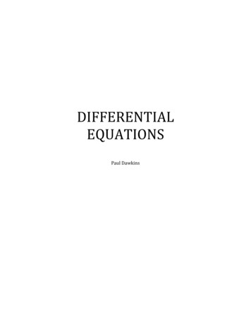
Chapter 1. Introduction1.41.4.113Origin of some equationsWave equationExample 1.4.1. Consider a string as a curve y u(x, t) (so it’s shape dependson time t) with a tension T and with a linear density ρ. We assume that ux 1.Observe that at point x the part of the string to the left from x pulls itup with a force F (x) : T ux .θx1x2Indeed, the force T is directed along the curve and the slope of angle θbetweenp the tangent to the curve and the horizontal line is ux ; so sin(θ) ux / 1 u2x which under our assumption we can replace by ux .Example 1.4.1 (continued). On the other hand, at point x the part of thestring to the right from x pulls it up with a force F (x) : T ux . Thereforethe total y-component of the force applied to the segment of the stringbetween J [x1 , x2 ] equalsZZF (x2 ) F (x1 ) x F (x) dx T uxx dx.JJRAccording to Newton’s law it must be equal to J ρutt dx where ρdx isthe mass and utt is the acceleration of the infinitesimal segment [x, x dx]:ZZρutt dx T uxx dx.JJSince this equality holds for any segment J, the integrands coincide:ρutt T uxx .(1.4.1)Example 1.4.2. Consider a membrane as a surface z u(x, y, t) with atension T and with a surface density ρ. We assume that ux , uyy 1.

Chapter 1. Introduction14Consider a domain D on the plane, its boundary L and a small segmentof the length ds of this boundary. Then the outer domain pulls this segmentup with the force T n · u ds where n is the inner unit normal to thissegment.Indeed, the total force is T ds but it pulls

Linear equations of order 2 (d)General theory, Cauchy problem, existence and uniqueness; (e) Linear homogeneous equations, fundamental system of solutions, Wron-skian; (f)Method of variations of constant parameters. Linear equations of order 2 with constant coe cients (g)Fundamental system of