WIXLIB

2Chapter 1 Introduction1.1 APPLICATIONS LEADING TO DIFFERENTIAL EQUATIONSIn order to apply mathematical methods to a physical or “real life” problem, we must formulate the problem in mathematical terms; that is, we must construct a mathematical model for the problem. Manyphysical problems concern relationships between changing quantities. Since rates of change are represented mathematically by derivatives, mathematical models often involve equations relating an unknownfunction and one or more of its derivatives. Such equations are differential equations. They are the subjectof this book.Much of calculus is devoted to learning mathematical techniques that are applied in later courses inmathematics and the sciences; you wouldn’t have time to learn much calculus if you insisted on seeinga specific application of every topic covered in the course. Similarly, much of this book is devoted tomethods that can be applied in later courses. Only a relatively small part of the book is devoted tothe derivation of specific differential equations from mathematical models, or relating the differentialequations that we study to specific applications. In this section we mention a few such applications.The mathematical model for an applied problem is almost always simpler than the actual situationbeing studied, since simplifying assumptions are usually required to obtain a mathematical problem thatcan be solved. For example, in modeling the motion of a falling object, we might neglect air resistanceand the gravitational pull of celestial bodies other than Earth, or in modeling population growth we mightassume that the population grows continuously rather than in discrete steps.A good mathematical model has two important properties: It’s sufficiently simple so that the mathematical problem can be solved. It represents the actual situation sufficiently well so that the solution to the mathematical problempredicts the outcome of the real problem to within a useful degree of accuracy. If results predictedby the model don’t agree with physical observations, the underlying assumptions of the model mustbe revised until satisfactory agreement is obtained.We’ll now give examples of mathematical models involving differential equations. We’ll return to theseproblems at the appropriate times, as we learn how to solve the various types of differential equations thatoccur in the models.All the examples in this section deal with functions of time, which we denote by t. If y is a functionof t, y 0 denotes the derivative of y with respect to t; thus,y0 Ddy:dtPopulation Growth and DecayAlthough the number of members of a population (people in a given country, bacteria in a laboratory culture, wildflowers in a forest, etc.) at any given time t is necessarily an integer, models that use differentialequations to describe the growth and decay of populations usually rest on the simplifying assumption thatthe number of members of the population can be regarded as a differentiable function P D P .t/. In mostmodels it is assumed that the differential equation takes the formP 0 D a.P /P;(1.1.1)where a is a continuous function of P that represents the rate of change of population per unit time perindividual. In the Malthusian model, it is assumed that a.P / is a constant, so (1.1.1) becomesP 0 D aP:(1.1.2)

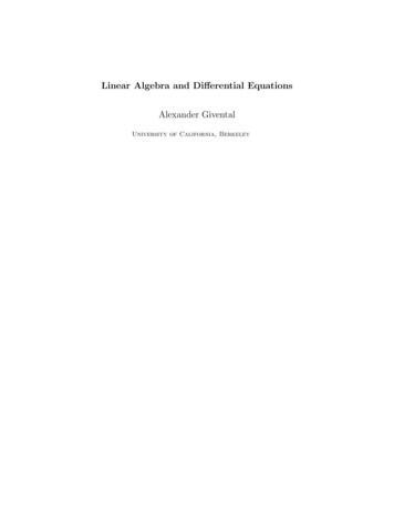
Section 1.1 Applications Leading to Differential Equations3(When you see a name in blue italics, just click on it for information about the person.) This modelassumes that the numbers of births and deaths per unit time are both proportional to the population. Theconstants of proportionality are the birth rate (births per unit time per individual) and the death rate(deaths per unit time per individual); a is the birth rate minus the death rate. You learned in calculus thatif c is any constant thenP D ce at(1.1.3)satisfies (1.1.2), so (1.1.2) has infinitely many solutions. To select the solution of the specific problemthat we’re considering, we must know the population P0 at an initial time, say t D 0. Setting t D 0 in(1.1.3) yields c D P .0/ D P0 , so the applicable solution isP .t/ D P0 e at :This implies thatlim P .t/ Dt !1 10if a 0;if a 0Ithat is, the population approaches infinity if the birth rate exceeds the death rate, or zero if the death rateexceeds the birth rate.To see the limitations of the Malthusian model, suppose we’re modeling the population of a country,starting from a time t D 0 when the birth rate exceeds the death rate (so a 0), and the country’sresources in terms of space, food supply, and other necessities of life can support the existing population. Then the prediction P D P0 e at may be reasonably accurate as long as it remains within limitsthat the country’s resources can support. However, the model must inevitably lose validity when the prediction exceeds these limits. (If nothing else, eventually there won’t be enough space for the predictedpopulation!)This flaw in the Malthusian model suggests the need for a model that accounts for limitations of spaceand resources that tend to oppose the rate of population growth as the population increases. Perhaps themost famous model of this kind is the Verhulst model, where (1.1.2) is replaced byP 0 D aP .1(1.1.4) P /;0where is a positive constant. As long as P is small compared to 1 , the ratio P P is approximatelyequal to a. Therefore the growth is approximately exponential; however, as P increases, the ratio P 0 Pdecreases as opposing factors become significant.Equation (1.1.4) is the logistic equation. You will learn how to solve it in Section 1.2. (See Exercise 2.2.28.) The solution isP0P D; P0 C .1 P0/e atwhere P0 D P .0/ 0. Therefore limt !1 P .t/ D 1 , independent of P0 .Figure 1.1.1 shows typical graphs of P versus t for various values of P0 .Newton’s Law of CoolingAccording to Newton’s law of cooling, the temperature of a body changes at a rate proportional to thedifference between the temperature of the body and the temperature of the surrounding medium. Thus, ifTm is the temperature of the medium and T D T .t/ is the temperature of the body at time t, thenT 0 D k.T(1.1.5)Tm /;where k is a positive constant and the minus sign indicates; that the temperature of the body increases withtime if it’s less than the temperature of the medium, or decreases if it’s greater. We’ll see in Section 4.2that if Tm is constant then the solution of (1.1.5) isT D Tm C .T0Tm /ekt;(1.1.6)

4Chapter 1 IntroductionP1/αtFigure 1.1.1 Solutions of the logistic equationwhere T0 is the temperature of the body when t D 0. Therefore limt !1 T .t/ D Tm , independent of T0 .(Common sense suggests this. Why?)Figure 1.1.2 shows typical graphs of T versus t for various values of T0 .Assuming that the medium remains at constant temperature seems reasonable if we’re considering acup of coffee cooling in a room, but not if we’re cooling a huge cauldron of molten metal in the sameroom. The difference between the two situations is that the heat lost by the coffee isn’t likely to raise thetemperature of the room appreciably, but the heat lost by the cooling metal is. In this second situation wemust use a model that accounts for the heat exchanged between the object and the medium. Let T D T .t/and Tm D Tm .t/ be the temperatures of the object and the medium respectively, and let T0 and Tm0 betheir initial values. Again, we assume that T and Tm are related by (1.1.5). We also assume that thechange in heat of the object as its temperature changes from T0 to T is a.T T0 / and the change in heatof the medium as its temperature changes from Tm0 to Tm is am .Tm Tm0 /, where a and am are positiveconstants depending upon the masses and thermal properties of the object and medium respectively. Ifwe assume that the total heat of the in the object and the medium remains constant (that is, energy isconserved), thena.T T0/ C am .Tm Tm0 / D 0:Solving this for Tm and substituting the result into (1.1.6) yields the differential equation aaT0 D k 1CT C k Tm0 CT0amamfor the temperature of the object. After learning to solve linear first order equations, you’ll be able toshow (Exercise 4.2.17) thatT DaT0 C am Tm0am .T0 Tm0 /Cea C ama C amk.1Ca am /t:

Section 1.1 Applications Leading to Differential Equations5TTmtFigure 1.1.2 Temperature according to Newton’s Law of CoolingGlucose Absorption by the BodyGlucose is absorbed by the body at a rate proportional to the amount of glucose present in the bloodstream.Let denote the (positive) constant of proportionality. Suppose there are G0 units of glucose in thebloodstream when t D 0, and let G D G.t/ be the number of units in the bloodstream at time t 0.Then, since the glucose being absorbed by the body is leaving the bloodstream, G satisfies the equationG 0 D G:(1.1.7)From calculus you know that if c is any constant thenG D ce t(1.1.8)satisfies (1.1.7), so (1.1.7) has infinitely many solutions. Setting t D 0 in (1.1.8) and requiring thatG.0/ D G0 yields c D G0 , soG.t/ D G0 e t :Now let’s complicate matters by injecting glucose intravenously at a constant rate of r units of glucoseper unit of time. Then the rate of change of the amount of glucose in the bloodstream per unit time isG 0 D G C r;(1.1.9)where the first term on the right is due to the absorption of the glucose by the body and the second termis due to the injection. After you’ve studied Section 2.1, you’ll be able to show (Exercise 2.1.43) that thesolution of (1.1.9) that satisfies G.0/ D G0 is rr tG D C G0e :

6Chapter 1 IntroductionGraphs of this function are similar to those in Figure 1.1.2. (Why?)Spread of EpidemicsOne model for the spread of epidemics assumes that the number of people infected changes at a rateproportional to the product of the number of people already infected and the number of people who aresusceptible, but not yet infected. Therefore, if S denotes the total population of susceptible people andI D I.t/ denotes the number of infected people at time t, then S I is the number of people who aresusceptible, but not yet infected. Thus,I 0 D rI.S I /;where r is a positive constant. Assuming that I.0/ D I0 , the solution of this equation isI DSI0I0 C .S I0 /erS t(Exercise 2.2.29). Graphs of this function are similar to those in Figure 1.1.1. (Why?) Since limt !1 I.t/ DS , this model predicts that all the susceptible people eventually become infected.Newton’s Second Law of MotionAccording to Newton’s second law of motion, the instantaneous acceleration a of an object with constant mass m is related to the force F acting on the object by the equation F D ma. For simplicity, let’sassume that m D 1 and the motion of the object is along a vertical line. Let y be the displacement of theobject from some reference point on Earth’s surface, measured positive upward. In many applications,there are three kinds of forces that may act on the object:(a) A force such as gravity that depends only on the position y, which we write as p.y/, wherep.y/ 0 if y 0.(b) A force such as atmospheric resistance that depends on the position and velocity of the object, whichwe write as q.y; y 0 /y 0 , where q is a nonnegative function and we’ve put y 0 “outside” to indicatethat the resistive force is always in the direction opposite to the velocity.(c) A force f D f .t/, exerted from an external source (such as a towline from a helicopter) thatdepends only on t.In this case, Newton’s second law implies thaty 00 Dq.y; y 0 /y 0p.y/ C f .t/;which is usually rewritten asy 00 C q.y; y 0 /y 0 C p.y/ D f .t/:Since the second (and no higher) order derivative of y occurs in this equation, we say that it is a secondorder differential equation.Interacting Species: CompetitionLet P D P .t/ and Q D Q.t/ be the populations of two species at time t, and assume that each populationwould grow exponentially if the other didn’t exist; that is, in the absence of competition we would haveP 0 D aPandQ0 D bQ;(1.1.10)where a and b are positive constants. One way to model the effect of competition is to assume thatthe growth rate per individual of each population is reduced by an amount proportional to the otherpopulation, so (1.1.10) is replaced byP0Q0DDaP QˇP C bQ;

Section 1.2 Basic Concepts7where and ˇ are positive constants. (Since negative population doesn’t make sense, this system worksonly while P and Q are both positive.) Now suppose P .0/ D P0 0 and Q.0/ D Q0 0. It canbe shown (Exercise 10.4.42) that there’s a positive constant such that if .P0 ; Q0 / is above the line Lthrough the origin with slope , then the species with population P becomes extinct in finite time, but if.P0 ; Q0 / is below L, the species with population Q becomes extinct in finite time. Figure 1.1.3 illustratesthis. The curves shown there are given parametrically by P D P .t/; Q D Q.t/; t 0. The arrowsindicate direction along the curves with increasing t.QLPFigure 1.1.3 Populations of competing species1.2 BASIC CONCEPTSA differential equation is an equation that contains one or more derivatives of an unknown function.The order of a differential equation is the order of the highest derivative that it contains. A differentialequation is an ordinary differential equation if it involves an unknown function of only one variable, or apartial differential equation if it involves partial derivatives of a function of more than one variable. Fornow we’ll consider only ordinary differential equations, and we’ll just call them differential equations.Throughout this text, all variables and constants are real unless it’s stated otherwise. We’ll usually usex for the independent variable unless the independent variable is time; then we’ll use t.The simplest differential equations are first order equations of the formdyD f .x/dxor, equivalently,y 0 D f .x/;where f is a known function of x. We already know from calculus how to find functions that satisfy thiskind of equation. For example, ify0 D x3;

8Chapter 1 IntroductionthenyDZx 3 dx Dx4C c;4where c is an arbitrary constant. If n 1 we can find functions y that satisfy equations of the formy .n/ D f .x/(1.2.1)by repeated integration. Again, this is a calculus problem.Except for illustrative purposes in this section, there’s no need to consider differential equations like(1.2.1).We’ll usually consider differential equations that can be written asy .n/ D f .x; y; y 0 ; : : : ; y .n1/(1.2.2)/;where at least one of the functions y, y 0 , . . . , y .n 1/ actually appears on the right. Here are someexamples:dyx2 D 0(first order);dxdyC 2xy 2 D2(first order);dxd 2ydyC2C y D 2x(second order);dx 2dxxy 000 C y 2 D sin x (third order);y .n/ C xy 0 C 3yD x(n-th order):Although none of these equations is written as in (1.2.2), all of them can be written in this form:y0y0y 00y 000y .n/D x2;D2 2xy 2 ;D 2x 2y 0 y;sin x y 2D;xD x xy 0 3y:Solutions of Differential EquationsA solution of a differential equation is a function that satisfies the differential equation on some openinterval; thus, y is a solution of (1.2.2) if y is n times differentiable andy .n/ .x/ D f .x; y.x/; y 0 .x/; : : : ; y .n1/.x//for all x in some open interval .a; b/. In this case, we also say that y is a solution of (1.2.2) on .a; b/.Functions that satisfy a differential equation at isolated points are not interesting. For example, y D x 2satisfiesxy 0 C x 2 D 3xif and only if x D 0 or x D 1, but it’s not a solution of this differential equation because it does notsatisfy the equation on an open interval.The graph of a solution of a differential equation is a solution curve. More generally, a curve C is saidto be an integral curve of a differential equation if every function y D y.x/ whose graph is a segmentof C is a solution of the differential equation. Thus, any solution curve of a differential equation is anintegral curve, but an integral curve need not be a solution curve.

Section 1.2 Basic Concepts9Example 1.2.1 If a is any positive constant, the circlex 2 C y 2 D a2is an integral curve of(1.2.3)x:yy0 D(1.2.4)To see this, note that the only functions whose graphs are segments of (1.2.3) areppy1 D a2 x 2 and y2 Da2 x 2 :We leave it to you to verify that these functions both satisfy (1.2.4) on the open interval . a; a/. However,(1.2.3) is not a solution curve of (1.2.4), since it’s not the graph of a function.Example 1.2.2 Verify that1x2C3x(1.2.5)xy 0 C y D x 2(1.2.6)yDis a solution ofon .0; 1/ and on . 1; 0/.Solution Substituting (1.2.5) andy0 D2x31x2into (1.2.6) yields0xy .x/ C y.x/ D x 2x31x2 C x21C3x D x2for all x 0. Therefore y is a solution of (1.2.6) on . 1; 0/ and .0; 1/. However, y isn’t a solution ofthe differential equation on any open interval that contains x D 0, since y is not defined at x D 0.Figure 1.2.1 shows the graph of (1.2.5). The part of the graph of (1.2.5) on .0; 1/ is a solution curveof (1.2.6), as is the part of the graph on . 1; 0/.Example 1.2.3 Show that if c1 and c2 are constants theny D .c1 C c2x/exC 2x(1.2.7)4is a solution ofy 00 C 2y 0 C y D 2x(1.2.8)on . 1; 1/.Solution Differentiating (1.2.7) twice yieldsy 0 D .c1 C c2 x/exC c2 exC2andy 00 D .c1 C c2x/ex2c2ex;

10 Chapter 1 Introductiony8642 2.0 1.5 1.0 0.50.51.01.52.0x 2 4 6 8Figure 1.2.1 y D1x2C3xsoy 00 C 2y 0 C yD .c1 C c2x/ex2c2exC2 Œ .c1 C c2x/e x C c2 e x C 2 C.c1 C c2 x/e x C 2x 4D .1 2 C 1/.c1 C c2x/e x C . 2 C 2/c2 eC4 C 2xx4 D 2xfor all values of x. Therefore y is a solution of (1.2.8) on . 1; 1/.Example 1.2.4 Find all solutions ofy .n/ D e 2x :(1.2.9)Solution Integrating (1.2.9) yieldse 2xC k1 ;2where k1 is a constant. If n 2, integrating again yieldsy .ny .n2/1/DDe 2xC k1 x C k2 :4If n 3, repeatedly integrating yieldsyDe 2xxn 1xn 2CkCkC C kn ;122n.n 1/Š.n 2/Š(1.2.10)

Section 1.2 Basic Concepts11where k1 , k2 , . . . , kn are constants. This shows that every solution of (1.2.9) has the form (1.2.10) forsome choice of the constants k1 , k2 , . . . , kn . On the other hand, differentiating (1.2.10) n times showsthat if k1 , k2 , . . . , kn are arbitrary constants, then the function y in (1.2.10) satisfies (1.2.9).Since the constants k1 , k2 , . . . , kn in (1.2.10) are arbitrary, so are the constantsk1.nk2;1/Š .n2/Š; ; kn :Therefore Example 1.2.4 actually shows that all solutions of (1.2.9) can be written asyDe 2xC c1 C c2 x C C cn x n2n1;where we renamed the arbitrary constants in (1.2

Elementary Differential Equations with Boundary Value Problems is written for students in science, en-gineering,and mathematics whohave completed calculus throughpartialdifferentiation. Ifyoursyllabus includes Chapter 10 (Linear Systems of Differential Equations), your