Transcription
Hindawi Publishing CorporationMathematical Problems in EngineeringVolume 2009, Article ID 238960, 35 pagesdoi:10.1155/2009/238960Review ArticleModeling Nonlinear Dynamics and Chaos:A ReviewLuis A. Aguirre1 and Christophe Letellier21Departamento de Engenharia Eletrônica da UFMG, Universidade Federal de Minas Gerais,Avenida Antônio Carlos 6627, 31270-901 Belo Horizonte, MG, Brazil2CORIA UMR 6614, Université de Rouen, Avenue de l’Université, BP 12,76801 Saint-Etienne du Rouvray Cedex, FranceCorrespondence should be addressed to Luis A. Aguirre, aguirre@cpdee.ufmg.brReceived 28 January 2009; Accepted 24 February 2009Recommended by Elbert E. Neher MacauThis paper reviews the major developments of modeling techniques applied to nonlinear dynamicsand chaos. Model representations, parameter estimation techniques, data requirements, and modelvalidation are some of the key topics that are covered in this paper, which surveys slightly overtwo decades since the pioneering papers on the subject appeared in the literature.Copyright q 2009 L. A. Aguirre and C. Letellier. This is an open access article distributed underthe Creative Commons Attribution License, which permits unrestricted use, distribution, andreproduction in any medium, provided the original work is properly cited.1. IntroductionThe field of nonlinear dynamics experienced a very quick and intense development in thelast thirty years or so. To determine the starting point of any subject is very difficult simplybecause we all stand on somebody elses showlders in any “new” attempt we make. For thesake of presentation, and because we feel that this understanding is not absurd anyway, theorigins of what we nowadays call the field of nonlinear dynamics can be traced back to thework of Henri Poincaré.In his studies on nonlinear dynamical systems Poincaré figured out that, since no analytical solution to most of nonlinear systems can be obtained, the whole set of solutions can beinvestigated in the so-called phase space spanned by the set of variables required for a complete description of states of the system 1 . A few years later, while investigating the threebody problem, he observed that small perturbations can deeply affect the solution 2 . Inorder to investigate nonlinear dynamics, Poincaré introduced the concepts of phase portrait,Poincaré section, periodic orbit, return map, bifurcation, fixed point, and so on. Most of theseconcepts were used by Andronov’s school in the 20 s 3 but the first representation in thephase space of a now called “chaotic solution” was due to the solution Edward Norton Lorenz 4 . The so-called Lorenz attractor thus represents the first chaotic attractor ever drawn.
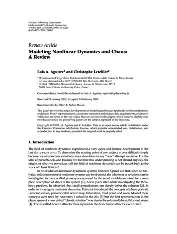
2Mathematical Problems in Engineering1400198719601980100Figure 1: Number of papers published per year up to 1994. The search machine used was ISI Web of Scienceusing Topic “nonlinear dynamics” OR chaos . Up to 1994 the total number of entries found was 8 400 shown in this figure . Up to 2008 the total number of entries is 39 180 and only in 2008 over 2 700 paperswere published within the topics nonlinear dynamics or chaos.From the publication of Lorenz’s paper up to the mid of the 70 s not many papers werepublished. Among those who contributed to the emergence of “chaos theory,” we can quoteRuelle and Takens paper on turbulence 5 , May about bifurcation 6 , Rössler’s new chaoticattractors 7 , Li and Yorke’s theorem for existence of chaos in map 8 . These contributions,published before 1980, popularized the word “chaos” as well as related techniques toinvestigate these new types of solutions.An important turning point happened around 1980 Figure 1 . There can be littledoubt that such a turning point was provoked, by the papers 9, 10 . The reason for thisis quite simple. So far, in the investigation of a nonlinear system ẋ f x , with f : Rm Rm ,typically it was assumed that the entire state vector x was available. This constraint wasclearly too restrictive in practical problems and consequently it was unclear what kind ofrole could the theory of nonlinear dynamics play in real world problems. From a suggestionby Ruelle, Packard and colleagues showed that it was possible to build a phase portrait forthe original system using a scalar s t h x , with h : Rm R 9 . Furthermore, Takensand Mañé mathematically proved under which conditions the phase space reconstructedusing s t was diffeomorphically equivalent to the one that would be obtained if the entirestate vector x was available 10, 11 . A decade later, other important works on the subjectwere published 12, 13 . When such works came to light, hopes of using the “new theory ofnonlinear dynamics” in practical problems were kindled, because now all that was required,in principle, and assuming an ideal measurement function was the recording of a singlevariable.When, in the early 1980, it became accepted that a scalar-reconstructed attractor couldbe equivalent to the original one, a great deal of work was devoted to developing tools toquantitatively characterize chaotic attractors. In the following decade, geometric measuressuch as dimensions 14, 15 , Lyapunov exponents 16 and entropies 17 were adapted,applied, and intensively investigated in the context of nonlinear dynamics. By the end ofthe 1980, there was a large set of works on these subjects as can be found in 18, 19 .Another turning point which can be detected in the number of papers published inthe field of nonlinear dynamics and chaos happened in the end of the decade 1980 Figure 1 .Unlike the turning point in the beginning of the decade, which quite clearly can be related tofundamental papers on embedding theory, it is quite hard to relate the turning point in thelate 1980 to a specific topic within the field. Most likely, such a turning point was an indicationthat several important topics started to be investigated as well as many applications started invarious fields. Among such topics we are to find the modeling of nonlinear dynamics and chaos.To survey the main developments of this topic is the aim of the present paper.
Mathematical Problems in Engineering32. Nonlinear System IdentificationBefore actually addressing how the modeling of nonlinear dynamics and chaos developedwithin the field, it is important to say that a significant amount of work was developedindependently, and sometimes previously, in the field of nonlinear system identification. Thebasic goals were very similar to those that later were pursued by the nonlinear dynamicscommunity but there were some important differences. Nonlinear system identification,which has its origins in the field of engineering, is usually concerned with nonautonomoussystems, discrete-time models, disturbance modeling this is vital to correctly deal with noisydata , and hardly ever was concerned with chaos. On the other hand, modeling nonlineardynamics and chaos, with its origins in physics and applied mathematics, usually concernedwith autonomous systems, very often considers continuous-time models, does not typicallymodel disturbances, and is strongly focused on chaotic systems.Having established such main distinctions between the two fields, let us point out thatthis paper is a survey of modeling techniques applied to nonlinear dynamics and chaos. Manysuch techniques have indeed been developed in the field of nonlinear system identificationand will be mentioned in this survey only to the extent in which they were applied tomodeling nonlinear dynamics and chaos. In the reminder of this section, for the sake ofcompletion, we present some issues in nonlinear system identification which will be relevantin the discussion of modeling techniques applied to nonlinear dynamic and chaos. In 20 the authors also point out some conceptual differences between what they call stochastic anddeterministic modeling.By the end of the 1970 linear system identfication was well established. The typicalproblem was to build a model, usually a transfer function of the formy k B q u k ,A q 2.1 from a set of possibly noisy data y k , u k , k 1, 2, . . . , N. In 2.1 A q and B q arepolynomials in the backward shift operator q 1 , that is, y k i q i y k . A commonly usedrepresentation of 2.1 is the ARX autoregressive model with exogeneous inputs modely k a1 y k 1 ··· any y k nyb1 u k 1 ···bnu u k nu , 2.2 where ny and nu are the maximum lags used. Noise is usually assumed to appear in theoutput y k . The presence and the type of noise usually are such that the standard leastsquares estimator will produce wrong results. This calls for disturbance modeling and sometype of generalized least squares algorithm, which is no longer a linear estimator. The simplesdisturbance model which is the moving average MA , which added to 2.2 , yields the wellknown ARMAX model. More general disturbance and system models have been proposedand studied in detail in standard texts such as 21, 22 .The approach to nonlinear system identification happened along different lines ofaction. One such line of action was to build so-called block-oriented models which consistedof a linear transfer function model see 2.1 either after or before a nonlinear staticfuntion g · , such were the Hammerstein and Wiener models. Another line of action wasthe development of nonparametric models like the Volterra models 23 . The numericalalgorithms involved in the development of such models were, in one way or another, related
4Mathematical Problems in Engineeringto the correlation function. A glimps of the state-of-the-art in the development of blockoriented and Volterra models at the end of 1970 can be found in 24 .A third, and last one to be mentioned here, line of action was to rewrite 2.2 as y k f y k 1 , . . . , y k ny , u k 1 , . . . , u k nu , 2.3 and to generalize for the case in which f · was a nonlinear function. Because the regressorvariables in 2.3 were of the ARX type, and because f · was now allowed to be nonlinear, 2.3 was referred to as a NARX model. As before, in the case of noisy data, disturbancemodeling is a must and, therefore, additional regressor terms of the MA moving average type have to be included in 2.3 . This lead to the now well-known acronym NARMAX. Thebuilding of a NARMAX model is typically composed of three steps: 1 the choice of theclass of models to be used for approximating f · . Some model classes include: polynomialmodels 25 , rational models 26 , neural models 27 , radial basis function models 28 , andwavelet networks 29 . 2 The following step is to determine which regressor variables touse in 2.3 , this is equivalent, although it is more general, to the choice of the embeddingspace in modeling nonlinear dynamics and chaos. For recent discussions and a survey onsuch techniques we refer the reader to 30–35 . 3 In model building the final step is toestimate whatever parameters f · may have. This step is far the easiest. Standard and robusttechniques for accomplishing parameter are available 21, 22 . The important problem ofmodel validation, which will be addressed later on, has more to do with model testing thanmodel building.3. Model Building for Nonlinear Dynamics and ChaosAfter presenting a brief introduction Section 1 and pointing out some standard problems innonlinear system identification Section 2 , we are ready to start surveying the developmentof data-driven models for nonlinear dynamics and chaos. There are various possible ways ofaddressing this vast subject, and it is not clear which will turn out to be the most pedagogicalone. We choose to start covering five of the earliest papers in the field and follow bydiscussing some of the mostly used model classes.3.1. A Few Pioneering WorksIn what follows, we begin by mentioning explicitly five pioneering works, the first four ofwhich were of great influence; 36–40 . The reason for including 40 in this group is its earlydate. In the remainder of the section we will survey some of the major developments in thefield. Together, these five papers have been quoted 2 719 times from their publication up tothe end of 2008. The search machine used was ISI Web of Science. 3.1.1. The Local Linear PredictorThe first papers on modeling nonlinear dynamics and chaos seem to have appeared in 1987.One of them is related to local linear modeling, the rest is generally concerned with someaspect of global modeling. Because of its historical importance, in this subsection, the mainpoints concerning the local linear predictor 36, 41 will be reviewed.
Mathematical Problems in Engineering5Suppose that a measured time series y 1 , y 2 , . . . , y N lies on a D-dimensionalattractor of an n th-order deterministic dynamical system. The starting point obtains anembedding from the recorded data. A convenient, though not unique, representation isachieved by using delay coordinates, for which a delay vector has the following form: T y k y k y k τ · · · y k de 1 τ , 3.1 where de is the embedding dimension and τ is the delay time. Takens has shown that embeddingswith de 2n will be faithful generically so that there is a smooth map f : Rde R such thaty k1 f y k 3.2 for all integers k, and where the forecasting time T and τ are also assumed to be integers.Takens’ theorem gives no indication as to how find. One of the first attempts to to build themap f from the data was the local linear predictor method, which started by partitioningnthe embedding space into neighbourhoods {Ui }Ni 1 within which the dynamics can bedeappropriately described by a linear map g : R R such thaty k1 gi y k for y k Ui , i 1, . . . , Nn . 3.3 Several choices for g have been suggested in the literature such as linear polynomials 36, 42 which can be interpolated to obtain an approximation of the map f 43 . Simplerchoices include zeroth-order approximations, also known as local constant predictors 36, 44 , anda weighted predictor 45 . Linsay proposed to weigh the predictions according to informationobtained from the local data 45 . In 46 the authors put forward the concept of pseudofalseneighbors which are left out from the construction of a local linear predictor to improveperformance, and in 47 the authors consider the multivariate case.A common difficulty of such approaches is that the data have to be separated intoneighbourhoods. Thus given a point in the embedded space the closest neighbours to such apoint must be found. It is well-known that for many methods most of the CPU time is spentin searching for close neighbours in the embedding space within the data 48 and that theeffort required to accomplish this grows exponentially with the embedding dimension.Another drawback has to do with model representation. The local linear predictordoes not have a closed form, in other words, it is not a global model. This prevents using theobtained model in any kind of analytical investigation.The local linear predictor has been applied to several real-time series including Wolf’ssunspot numbers 20, 49 , daily dollar exchange rates 50 , R-R heart intervals 49 , tomention a few.3.1.2. Equations of MotionIn 1987 James Crutchfield and Bruce McNamara published a paper that became a reference inthe field 37 . The title of this section is a reference to that paper rather to a particular class ofmodels. It seems safe to say that this was the first journal paper in the field devoted to globalmodeling, as oposed to the “patchwork-models” produced by the local linear approach, andwhich the authors call the “atlas equation of motion procedure.”
6Mathematical Problems in Engineering x , withIn 37 the authors consider linear-in-the-parameter models of the type x F T x , where φ is a vector of function basis and A is a vector of parameters to x A φ F be estimated from data. Discrete-time models are also considered in the paper. The authorsdescribed their method without any particular class of function basis in mind. The parametervector was estimated using a singular value decomposition implementation of least squares.Their method is general and quite basic: the embedding dimension and the number of basisfunctions used are varied over a set of alternatives. The choosen model is the one withsmallest entropy I M . In their examples, that include the Hénon map, Duffing, and vander Pol oscillators, the function basis used was B-splines and discrete monomials.In closing, it should be said that more than a method, Crutchfield and McNamaraput forward a general philosophy for modeling chaotic data. With the exception of someissues that are specific to such data, their procedure does not differ substantially from worksin the field of nonlinear system identification using linear-in-the-parameter models widelyavailable at that time see 34 for a survey .3.1.3. Multivariable Functional InterpolationThe paper by David Broomhead and David Lowe is among the four pioneering works that wehave selected to start surveying the main developments in modeling of nonlinear dynamicsand chaos 38 . Such a paper is often quoted as being responsible for the proposition ofusing Radial Basis Function RBF models to describe nonlinear systems. Although in theirpaper the authors quote a review work by M. J. D. Powell entitled “Radial basis functionsfor multivariable interpolation: a review,” it seems that the work by Powell did not considerdynamical systems but only static problems.A typical model, as proposed by Broomhead and Lowe, can be written asy k b0p ωi φ x k 1 c , 3.4 i 1where p is the number of radial basis functions, φ, b0 , and wi are the unknown parameters tobe estimated, c are the centers, and · is usually the Euclidean norm. As it will be seen in thenext section, Martin Casdagli also worked with RBF models, as pointed out by Broomwheadand Lowe: “We note that in this application our approach is very close to that of Casdagliwho has applied radial basis functions to the construction of nonlinear maps from time seriesdata. Here the authors quote Casdagli’s paper as “submitted to Physica D.” That paper, thatwill be mentioned in the next section, was eventually published in 1989. Unlike Casdagliwho used strict interpolation, we will employ the least squares generalization.” By “strictinterpolation” the authors mean that the number of unknowns parameters and constraints built from data is the same more on this in Section 3.1.4 .This paper is curious in some aspects. First of all, it is clearly devoted to machinelearning for purposes of classification. Several pages are devoted to the problem ofapproximating the exclusive-OR function. The last examples in the paper seem to be anafterthought and consist of the modeling of the doubling map xn 1 2xn modulo 1 andof the quadratic map xn 1 4xn 1 xn . Also, only three works are listed in the referenceswhich are related to modeling nonlinear dynamics and chaos: 36, 39 and a preprint byLapedes and Farber 51 . Such a manuscript was at the time submitted to Proceedings of theIEEE. It seems that this paper was never published as such, but has circulated as a technical
Mathematical Problems in Engineering7report. This report is cited by a number of early papers on modeling nonlinear dynamics andchaos, proving to have been quite influential. It is also very curious that no paper or resulton embedding theory was used by Broomhead and Lowe. Because both their examples use1D maps, there was no need for any serious embedding. In summary, the contribution of 38 seems to be the suggestion of using RBF models for nonlinear dynamics, but for the generalview of the embedding-modeling problem we should look into 37 as the pioneering work.The fusion of such papers, that is, the use of RBF models in an embedding environment tomodel and predict nonlinear dynamics, happened in the next paper to be considered.3.1.4. Prediction of Chaotic Time SeriesFrom the abstract of the paper we clearly read the objective of the paper: “numericaltechniques are presented for constructing nonlinear predictive models directly from timeseries data” 39 . The basic motivation for such was to “convincingly distinguish lowdimensional chaos from randomness.” In fact, Casdagli argues in favor of his model-basedapproach when comparing it with the use of dimension calculations and Lyapunov exponentsto distinguish noise from chaos.With respect to the model class, this paper is remarkable because it comparedpolynomial, rational, and RBF models, plus local linear predictions. Very few papers presentresults for more than one model class, a more recent exception to this rule is 52 .As for the use of “strict interpolation” Broomhead and Lowe or simply “interpolants” Casdagli or “approximants” Casdagli , the situation is not completely clear. Thepaper mentions both. When describing general techniques polynomial and rational models ,Casdagli mentions the least squares solution. However, when presenting the RBF model theonly case considered is that of choosing the model structure so as to have an inverse problemwith unique solution. At the end of that section, the least squares solution is mentionedagain, but as “ongoing research.” One of the critical problems of the “strict interpolation”approach is the total lack of robustness to noise. In fact, Casdagli does not consider anynoise in the “global modeling” examples, but only in the “distinguishing noise from chaos”examples. In two occasions interesting remarks are made. In discussing modeling difficultiesCasdagli says: “this does not appear to be due to numerical errors in the least-squares fittingand matrix inversion algorithms” 39, page 343 . This gives the impression that he wasactually implementing both: the least-squares algorithm to fit approximants and the matrixinversion algorithm to find the solution to the strict interpolation problem . The first wasprobably related to polynomial and rational models and the latter to RBF models. The secondcase, when discussing the use of RBF models for predicting invariant measures, the numberof data points is quoted as N 25 and the data were noise-free. This clearly suggests “strictinterpolation.”The RBF models considered by Casdagli were of the form compare with 3.4 y k N 1 i 1ωi φ x k 1 c d μn pn x , 3.5 n 1where N is the number of data iterates, pn is a basis of the space of polynomials of degreeat most d from Rn to R, with d known, and μn are parameters. The author points out that“frequently the polynomial term is not included,” which is interesting in the light of otherresults, to be mentioned in Section 3.2.3.
8Mathematical Problems in EngineeringCasdagli investigated the accuracy of short-term predictions based on model iterationand the direct method, which amounts to fitting a predictor with a single prediction horizonequivalent to the various one-step-ahead predictions of the iterative method. In the variouscases investigated, the iterative method proved superior. A similar aim was pursued in thecontext of neural networks in 53 , in the context of Volterra expansions in 54 and using akernel-based approach in 43 . Finally, the author showed that the fitted RBF models werecapable of reproducing some invariants, such as Poincaré sections and bifurcation diagrams.Although he only considered the noise-free case, a very significant step towards seriousmodel validation was given. Perhaps the greatest lack in this relevant paper is that there is nomention on structure selection. Model instability under iteration is prematurely attributed tothe model class and not to an unsuitable model structure.By model class we mean the type of models used, as for instance polynomials, RBFsor neural networks. By model structure we mean the model topology, of a particular class.For instance, in the case of RBF models, the model structure is determined by the type andnumber of basis functions used, the lags used to compose the input space, and so on.3.1.5. Construction of Differential EquationsThe early paper by Cremers and Hübler had the clear objective to “obtain a concisedescription of an observed chaotic time sequence” 40 . From the beginning, the authors wereclearly concerned with chaotic data. The model class they considered was a basis of Legendrepolynomials, and in the introduction of the paper it was stated that the true objective was toestimate the parameters of a differential equation. This more restricted aim was confirmedlater in 55 .The authors discuss a few aspects of embedding and the effect of dynamical noise. Intheir numerical examples no noise is considered. They mention sucessful estimation of theparameters for two systems: Lorenz and an autonomous version of the van der Pol oscillator,for which the following 4th-order approximation was used:ẋj l m 4cj,l,m P l x1 P m x2 ,j 1, 2, 3.6 l,m 0where cj,l,m are the parameters to be estimated. The Legendre polynomials P l x1 and P m x2 must be evaluated at x1 and x2 , in addition to the time derivatives of x1 and x2 at each pointin state space considered. The derivatives were estimated numerically, but there is no clearindication as to how this was accomplished nor what would be the effect on such estimates ofmeasurement noise which they considered not . The authors justify the use of a polynomialexpansion by stating “if nothing is known about the properties of the flow vector field, a fit bya polynom sic series is frequently favourable” 40, page 800 . This last remark results froma general theorem by Weierstrass stating that any analytical function can be approximated byan infinite polynomial expansion.Breeden and Hübler later remarked that the 1987 paper also considered the discretetime case, which is definitely not obvious. Then, so far the field of nonlinear dynamicsis concerned, this paper seems to mark the beginning of building differential polynomialequations from data. Although no mention on important practical issues is made in thispaper, such as structure selection, derivative and parameter estimation, it has the merit ofhaving opened the way for a prosperous modeling class of techniques, to be surveyed inSection 3.2.1.
Mathematical Problems in Engineering9The citation relationships among these five pioneering papers are illustrated inFigure 2. In the center of the diagram the embedding papers 9, 10 appear as a commonfeature, with the exception of the paper 38 see discussion in Section 3.1.3 . This quotationdiagram suggests that Cremers and Hübler were not aware of the other papers on modelbuilding. Their paper was submitted in September 1986. It is interesting to notice notshown in the diagram that Broomhead & Lowe and Casdagli mention the work of Lapedesand Farber see 51 .3.2. Model ClassesIn the description to follow, the order of the model classes mentioned is somewhat arbitrary.We follow a rough chronological order of the first papers in each class.3.2.1. Continuous-Time PolynomialsA number of papers appeared in the early nineties which had as a common goal fittingordinary differential equations ODEs to observed data. As pointed out in Section 3.1.5, thepaper 40 was pioneering in this field, although it did not deal with any practical issue.Unlike Cremers and Hübler, most papers that followed, instead of using a basis of Legendrepolynomials, used “Taylor-series expansions.” As an example, such an expansion for a 2Dsystem is 56 ẋ f x, y a00 a10 x ẏ g x, y b00 b10 ya01 ya11 xy···aij xi yj··· ,b01 xb11 xy···bij xj yi··· . 3.7 A similar representation was used by Gouesbet who started investigating under whichconditions it was possible to reconstruct the vector field X, Y, Z from a single measurementX x of an original vector field x, y, z 57, 58 . The reconstructed system was expressed asẊ Y,Ẏ Z, 3.8 Ż F X, Y, Z ,and both polynomial and rational expansions for F were investigated. The polynomialexpansions of F used were equivalent to 3.7 . Although no reconstruction from data wasperformed in that paper, the challenge was acknowledged and pursued shortly after 59 .In the last paper, the important issue of estimating the derivatives based on finite-differenceschemes from data was considered. This was an important step towards dealing with realdata but a key hurdle still had to be transposed: measurement noise. To do this was one ofthe key objectives in 60 , where this global modeling technique finally reached maturity. Aspointed out in an early paper “noise removal · · · is required because standard systems · · · rely on derivative evaluations” 58, page 1795 , to deal with noise was to remove it from thedata, not so much as for discrete-time modeling techniques which are made to cope withnoise.Other polynomial expansions are to be found in the literature. Giona and colleaguesinvestigated the use of a basis of polynomials to approximate both continuous-time and
10Mathematical Problems in ckard et e 2: Quotation diagram. A B indicates that A quotes B. The indicates that only paper 10 wasquoted. Also, Crutchfield and McNamara quoted Farmer and Sidorowich’s paper as the technical report:Preprint LA-UR-87-1502.discrete-time dynamical systems 61 . In both cases the system was approximated by a linearcombination of such polynomial functions which are obtained “from the knowledge of thehierarchy of moments.” The procedure is quite involved, and long data sets are required toestimate the parameters. In their examples, N 5 104 was used for the Hénon and Ikedamaps, and N 4 105 was used for the Lorenz system.Practical implementation of global modelling using continuous-time model requiresan integration scheme. For instance, the explicit Euler integration schemeyn1 yn 3.9
using Topic “nonlinear dynamics” OR chaos . Up to 1994 the total number of entries found was 8400 shown in this figure . Up to 2008 the total number of entries is 39180 and only in 2008 over 2700 papers were published within the topics
