WIXLIB

viCONTENTS6.7Kac Ring Model . . . . . . . . . . . . . . . . . . . . . . . . . . . . . . . . .1786.8Remarks on Ergodic Theory . . . . . . . . . . . . . . . . . . . . . . . . . .1826.8.1The microcanonical ensemble. . . . . . . . . . . . . . . . . . . . .1836.8.2Ergodicity and mixing . . . . . . . . . . . . . . . . . . . . . . . . .1847 Maps, Strange Attractors, and Chaos1897.1Maps . . . . . . . . . . . . . . . . . . . . . . . . . . . . . . . . . . . . . . .1897.2One-dimensional Maps . . . . . . . . . . . . . . . . . . . . . . . . . . . . . .1927.2.1Lyapunov Exponents . . . . . . . . . . . . . . . . . . . . . . . . . .1957.2.2Chaos in the logistic map . . . . . . . . . . . . . . . . . . . . . . . .1957.2.3Intermittency . . . . . . . . . . . . . . . . . . . . . . . . . . . . . .1977.3Attractors . . . . . . . . . . . . . . . . . . . . . . . . . . . . . . . . . . . . .1977.4The Lorenz Model . . . . . . . . . . . . . . . . . . . . . . . . . . . . . . . .1987.4.1Fixed point analysis . . . . . . . . . . . . . . . . . . . . . . . . . . .2007.4.2Poincaré section . . . . . . . . . . . . . . . . . . . . . . . . . . . . .2027.4.3Rössler System203. . . . . . . . . . . . . . . . . . . . . . . . . . . . .8 Front Propagation8.18.28.3207Reaction-Diffusion Systems . . . . . . . . . . . . . . . . . . . . . . . . . . .2078.1.1Single component systems . . . . . . . . . . . . . . . . . . . . . . .2078.1.2Propagating front solutions . . . . . . . . . . . . . . . . . . . . . . .2088.1.3Fisher’s equation . . . . . . . . . . . . . . . . . . . . . . . . . . . .2118.1.4Velocity selection and stability . . . . . . . . . . . . . . . . . . . . .2118.1.5Stability calculation . . . . . . . . . . . . . . . . . . . . . . . . . . .213Multi-Species Reaction-Diffusion Systems . . . . . . . . . . . . . . . . . . .2158.2.1Propagating front solutions . . . . . . . . . . . . . . . . . . . . . . .217Excitable Media . . . . . . . . . . . . . . . . . . . . . . . . . . . . . . . . .2208.3.1222Front propagation in excitable media . . . . . . . . . . . . . . . . .9 Pattern Formation227

viiCONTENTS9.0.2Reaction-Diffusion Dynamics Revisited . . . . . . . . . . . . . . . .2279.1Turing and Hopf Instabilities . . . . . . . . . . . . . . . . . . . . . . . . . .2299.2The Brusselator . . . . . . . . . . . . . . . . . . . . . . . . . . . . . . . . .2309.2.1. . . . . . . . . . . . . . . . . . . . . . . .2329.3Rayleigh-Bénard Instability . . . . . . . . . . . . . . . . . . . . . . . . . . .2359.4Center Manifold Reduction . . . . . . . . . . . . . . . . . . . . . . . . . . .2379.5Selection and Stability of Spatial Patterns . . . . . . . . . . . . . . . . . . .2399.5.1d 1 . . . . . . . . . . . . . . . . . . . . . . . . . . . . . . . . . . .2399.5.2Remarks on the amplitude equations for d 1 . . . . . . . . . . . .2409.5.3d 2 . . . . . . . . . . . . . . . . . . . . . . . . . . . . . . . . . . .2419.5.4d 3 . . . . . . . . . . . . . . . . . . . . . . . . . . . . . . . . . . .2489.6Anisotropy . . . . . . . . . . . . . . . . . . . . . . . . . . . . . . . . . . . .2489.7Phase Diffusion : Eckhaus and Zigzag Instabilities . . . . . . . . . . . . . .249The amplitude equation10 Solitons25310.1 The Korteweg-deVries Equation . . . . . . . . . . . . . . . . . . . . . . . .25410.1.1KdV solitons . . . . . . . . . . . . . . . . . . . . . . . . . . . . . . .25510.1.2Periodic solutions : soliton trains . . . . . . . . . . . . . . . . . . .25610.1.3Interlude: primer on elliptic functions . . . . . . . . . . . . . . . . .25710.1.4The soliton lattice . . . . . . . . . . . . . . . . . . . . . . . . . . . .25810.1.5N -soliton solutions to KdV . . . . . . . . . . . . . . . . . . . . . . .25910.1.6Bäcklund transformations . . . . . . . . . . . . . . . . . . . . . . .26310.2 Sine-Gordon Model . . . . . . . . . . . . . . . . . . . . . . . . . . . . . . .26610.2.1Tachyon solutions . . . . . . . . . . . . . . . . . . . . . . . . . . . .26810.2.2Hamiltonian formulation . . . . . . . . . . . . . . . . . . . . . . . .26810.2.3Phonons . . . . . . . . . . . . . . . . . . . . . . . . . . . . . . . . .26910.2.4Mechanical realization . . . . . . . . . . . . . . . . . . . . . . . . .27010.2.5Kinks and antikinks . . . . . . . . . . . . . . . . . . . . . . . . . . .27010.2.6Bäcklund transformation for the sine-Gordon system . . . . . . . .271

viiiCONTENTS10.3 Nonlinear Schrödinger Equation . . . . . . . . . . . . . . . . . . . . . . . .27410.3.1Amplitude-phase representation . . . . . . . . . . . . . . . . . . . .27410.3.2Phonons . . . . . . . . . . . . . . . . . . . . . . . . . . . . . . . . .27510.3.3Soliton solutions for NLS( ) . . . . . . . . . . . . . . . . . . . . . .27610.3.4Dark solitons for NLS( ) . . . . . . . . . . . . . . . . . . . . . . . .27711 Shock Waves27911.1 Nonlinear Continuity Equation . . . . . . . . . . . . . . . . . . . . . . . . .27911.2 Shocks . . . . . . . . . . . . . . . . . . . . . . . . . . . . . . . . . . . . . . .28511.3 Internal Shock Structure . . . . . . . . . . . . . . . . . . . . . . . . . . . .28611.3.1Quadratic J(ρ) . . . . . . . . . . . . . . . . . . . . . . . . . . . . .28711.4 Shock Fitting . . . . . . . . . . . . . . . . . . . . . . . . . . . . . . . . . . .28811.4.1An Important Caveat . . . . . . . . . . . . . . . . . . . . . . . . . .28811.4.2Recipe for shock fitting (J ′′′ (ρ) 0) . . . . . . . . . . . . . . . . . .28911.4.3Example problem . . . . . . . . . . . . . . . . . . . . . . . . . . . .29011.5 Long-time Behavior of Shocks. . . . . . . . . . . . . . . . . . . . . . . . .29311.5.1Fate of a hump . . . . . . . . . . . . . . . . . . . . . . . . . . . . .29311.5.2N-wave and P-wave . . . . . . . . . . . . . . . . . . . . . . . . . . .29511.6 Shock Merging . . . . . . . . . . . . . . . . . . . . . . . . . . . . . . . . . .29611.7 Shock Fitting for General J(ρ) . . . . . . . . . . . . . . . . . . . . . . . . .29711.8 Sources . . . . . . . . . . . . . . . . . . . . . . . . . . . . . . . . . . . . . .29811.8.1Examples . . . . . . . . . . . . . . . . . . . . . . . . . . . . . . . . .29911.8.2Moving sources . . . . . . . . . . . . . . . . . . . . . . . . . . . . .29911.9 Burgers’ Equation . . . . . . . . . . . . . . . . . . . . . . . . . . . . . . . .30011.9.1The limit ν 0 . . . . . . . . . . . . . . . . . . . . . . . . . . . . .30111.9.2Examples . . . . . . . . . . . . . . . . . . . . . . . . . . . . . . . . .30311.9.3Confluence of shocks . . . . . . . . . . . . . . . . . . . . . . . . . .30511.10 Appendix I : The Method of Characteristics . . . . . . . . . . . . . . . . . .30711.10.1 Example . . . . . . . . . . . . . . . . . . . . . . . . . . . . . . . . .307

CONTENTS11.11 Appendix II : Shock Fitting an Inverted Parabola . . . . . . . . . . . . . .ix308

x0.1CONTENTSPrefaceThis is a proto-preface. A more complete preface will be written after these notes arecompleted.These lecture notes are intended to supplement a graduate level course in nonlinear dynamics.

Chapter 0Reference MaterialsNo one book contains all the relevant material. Here I list several resources, arranged bytopic. My personal favorites are marked with a diamond ( ).0.1Dynamical Systems S. Strogatz, Nonlinear Dynamics and Chaos (Addison-Wesley, 1994) S. Neil Rasband, Chaotic Dynamics of Nonlinear Systems (Wiley, 1990) J. Guckenheimer and P. Holmes, Nonlinear Oscillations, Dynamical Systems, and Bifurcations of Vector Fields (Springer, 1983) E. A. Jackson, Perspectives of Nonlinear Dynamics, 2 vols. (Cambridge, 1991) A. J. Lichtenberg and M. A. Lieberman, Regular and Stochastic Motion (Springer,1983) R. Z. Sagdeev, D. A. Usikov, and G. M. Zaslavsky, Nonlinear Physics from the Pendulum to Turbulence and Chaos (Harwood Academic, 1988) M. Lakshmanan and S. Rajasekar, Nonlinear Dynamics : Integrability, Chaos, andPatterns (Springer, 2003) H. G. Schuster and W. Just, Deterministic Chaos, 4th ed. (Wiley-VCH, 2005)1

2CHAPTER 0. REFERENCE MATERIALS M. Tabor, Chaos and Integrability in Nonlinear Dynamics (Wiley, 1989) E. Ott, Chaos in Dynamical Systems, 2nd ed. (Cambridge, 2002)0.2Hamiltonian Mechanics G. M. Zaslavsky, Hamiltonian Chaos and Fractional Dynamics (Oxford, 2005) J. V. José and E. J. Saletan, Classical Dynamics : A Contemporary Approach (Cambridge, 1998) V. I. Arnold, V. V. Kozlov, and A. I. Neishtadt, Mathematical Aspects of Classicaland Celestial Mechanics (Springer, 2006) A. L. Fetter and J. D. Walecka, Nonlinear Mechanics (Dover, 2006) I. Percival and D. Richards, Introduction to Dynamics (Cambridge, 1982)0.3Differential Equations D. Zwillinger, Handbook of Differential Equations, 3rd ed. (Academic Press, 1998) A. H. Nayfeh, Introduction to Perturbation Techniques (Wiley, 1981) C. M. Bender and S. A. Orszag, Advanced Mathematical Methods for Scientists andEngineers (Springer, 1999) V. I. Arnold, Ordinary Differential Equations (MIT Press, 1973) V. I. Arnold, Geometrical Methods in the Theory of Ordinary Differential Equations(Springer, 1988) L. Perko, Differential Equations and Dynamical Systems, 3rd ed. (Springer, 2001)

0.4. SYNCHRONIZATION3 J. A. Sanders and F. Verhulst, Averaging Methods in Nonlinear Dynamical Systems(Springer, 1985).0.4Synchronization Y. Kuramoto, Chemical Oscillations, Waves, and Turbulence (Dover, 2003) A. Pikovsky, M. Rosenblum, and J. Kurths, Synchronization : A Universal Conceptin Nonlinear Sciences (Cambridge, 2001)0.5Nonlinear Wave Equations G. B. Whitham, Linear and Nonlinear Waves (Wiley, 1999) A. Scott, Nonlinear Science, 2nd ed. (Oxford, 2003) E. Infeld and G. Rowlands, Nonlinear Waves, Solitons, and Chaos (Cambridge, 2000) R. Rajaraman, Solitons and Instantons (North-Holland, 1987) H.-K. Rhee, R. Aris, and N. R. Amundson, First-Order Partial Differential Equations(2 vols.) (Dover, 1986) L. I. Pismen, Vortices in Nonlinear Fields (Oxford, 1999)0.6Pattern Formation P. Manneville, Instabilities, Chaos, and Turbulence (Imperial College Press, 2004) D. Walgraef, Spatio-Temporal Pattern Formation (Springer, 1996) P. Manneville, Dissipative Structures and Weak Turbulence (Academic Press, 1990)

4CHAPTER 0. REFERENCE MATERIALS L. M. Pismen, Patterns and Interfaces in Dissipative Dynamics (Springer, 2006) M. I. Rabinovich, A. B. Ezersky, and P. D. Weidman, The Dynamics of Patterns(World Scientific, 2000) R. Hoyle, Pattern Formation : An Introduction to Methods (Cambridge, 2006)0.7Biological Applications J. D. Murray, Mathematical Biology, (3rd ed., 2 vols.) (Springer, 2002) E. M. Izhikevich, Dynamical Systems in Neuroscience (MIT Press, 2007) L. Edelstein-Keshet, Mathematical Models in Biology (SIAM, 2005) J. Hofbauer and K. Sigmund, Evolutionary Games and Population Dynamics (Cambridge, 1998) M. A. Nowak, Evolutionary Dynamics (Harvard, 2006)

Chapter 1Dynamical Systems1.11.1.1IntroductionPhase space and phase curvesDynamics is the study of motion through phase space. The phase space of a given dynamicalsystem is described as an N -dimensional manifold, M. A (differentiable) manifold M is atopological space that is locally diffeomorphic to RN .1 Typically in this course M will RNitself, but other common examples include the circle S1 , the torus T2 , the sphere S2 , etc.Let gt : M M be a one-parameter family of transformations from M to itself, withgt 0 1, the identity. We call gt the t-advance mapping. It satisfies the composition rulegt gs gt s .(1.1)Let us choose a point ϕ0 M. Then we write ϕ(t) gt ϕ0 , which also is in M. The set gt ϕ0 t R , ϕ0 M is called a phase curve. A graph of the motion ϕ(t) in the productspace R M is called an integral curve.1.1.2Vector fieldsThe velocity vector V (ϕ) is given by the derivativeV (ϕ) ddtgt ϕ .(1.2)t 0The velocity V (ϕ) is an element of the tangent space to M at ϕ, abbreviated TMϕ .If M is N -dimensional, then so is each TMϕ (for all p). However, M and TMϕ may1A diffeomorphism F : M N is a differentiable map with a differentiable inverse. This is a specialtype of homeomorphism, which is a continuous map with a continuous inverse.5

6CHAPTER 1. DYNAMICAL SYSTEMSFigure 1.1: An example of a phase curve.differ topologically. For example, if M S1 , the circle, the tangent space at any point isisomorphic to R.For our purposes, we will take ϕ (ϕ1 , . . . , ϕN ) to be an N -tuple, i.e. a point in RN . Theequation of motion is then dϕ(t) V ϕ(t) .(1.3)dtNote that any N th order ODE, of the general form dxdN 1xdNx F x, , . . . , N 1 ,dtNdtdt(1.4)may be represented by the first order system ϕ̇ V (ϕ). To see this, define ϕk dk 1x/dtk 1 , with k 1, . . . , N . Thus, for j N we have ϕ̇j ϕj 1 , and ϕ̇N f .In other words,ϕ̇z } ϕ .1.d . dt ϕV (ϕ)} { { z ϕ2 . . . ϕ N 1N F ϕ1 , . . . , ϕNϕN1.1.3(1.5)Existence / uniqueness / extension theoremsTheorem : Given ϕ̇ V (ϕ) and ϕ(0), if each V (ϕ) is a smooth vector field over someopen set D M, then for ϕ(0) D the initial value problem has a solution on somefinite time interval ( τ, τ ) and the solution is unique. Furthermore, the solution has aunique extension forward or backward in time, either indefinitely or until ϕ(t) reaches theboundary of D.Corollary : Different trajectories never intersect!

71.1. INTRODUCTION1.1.4Linear differential equationsA homogeneous linear N th order ODE,dN 1xdxdNx c0 x 0 c . . . c1N 1NN 1dtdtdt(1.6)may be written in matrix form, as ϕ1 d ϕ2 . dt . ϕNThus,Mz 00.} 0 ···1 ···.10.00. c0 c1 c2 · · · cN 1 { ϕ1 ϕ 2 . . . (1.7)ϕNϕ̇ M ϕ ,(1.8)and if the coefficients ck are time-independent, i.e. the ODE is autonomous, the solution isobtained by exponentiating the constant matrix Q:ϕ(t) exp(M t) ϕ(0) ;(1.9)the exponential of a matrix may be given meaning by its Taylor series expansion. If theODE is not autonomous, then M M (t) is time-dependent, and the solution is given bythe path-ordered exponential,ϕ(t) P exp( Zt)dt′ M (t′ ) ϕ(0) ,0(1.10)As defined, the equation ϕ̇ V (ϕ) is autonomous, since gt depends only on t and on noother time variable. However, by extending the phase space from M to R M, which is ofdimension (N 1), one can describe arbitrary time-dependent ODEs.1.1.5Lyapunov functionsFor a general dynamical system ϕ̇ V (ϕ), a Lyapunov function L(ϕ) is a function whichsatisfies L(ϕ) · V (ϕ) 0 .(1.11)There is no simple way to determine whether a Lyapunov function exists for a given dynamical system, or, if it does exist, what the Lyapunov function is. However, if a Lyapunovfunction can be found,then this severely limits the possible behavior of the system. This is because L ϕ(t) must be a monotonic function of time: dϕdL ϕ(t) L · L(ϕ) · V (ϕ) 0 .dtdt(1.12)

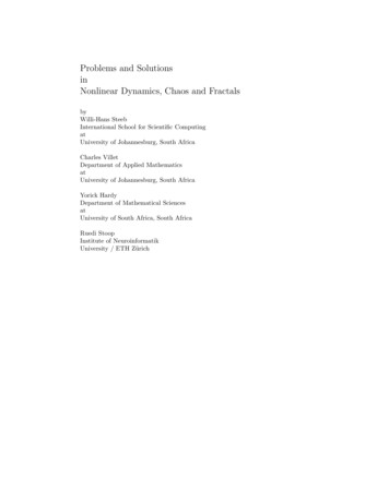
8CHAPTER 1. DYNAMICAL SYSTEMSThus, the system evolves toward a local minimum of the Lyapunov function. In generalthis means that oscillations are impossible in systems for which a Lyapunov function exists.For example, the relaxational dynamics of the magnetization M of a system are sometimesmodeled by the equation FdM Γ,(1.13)dt Mwhere F (M, T ) is the free energy of the system. In this model, assuming constant temper 2ature T , Ḟ F ′ (M ) Ṁ Γ F ′ (M ) 0. So the free energy F (M ) itself is a Lyapunovfunction, and it monotonically decreases during the evolution of the system. We shall meetup with this example again in the next chapter when we discuss imperfect bifurcations.1.2N 1 SystemsWe now study phase flows in a one-dimensional phase space, governed by the equationdu f (u) .dt(1.14)Again, the equation u̇ h(u, t) is first order, but not autonomous, and it corresponds tothe N 2 system, d uh(u, t) .(1.15)1dt tThe equation 1.14 is easily integrated:du dtf (u) t t0 Zuu0du′f (u′ ).(1.16)This gives t(u); we must then invert this relationship to obtain u(t).Example : Suppose f (u) a bu, with a and b constant. Thendt du b 1 d ln(a bu)a bu! whence1t lnba b u(0)a b u(t)u(t) a a exp( bt) . u(0) bb(1.17)(1.18)Even if one cannot analytically obtain u(t), the behavior is very simple, and easily obtainedby graphical analysis. Sketch the function f (u). Then note that f (u) 0 u̇ 0 move to right(1.19)u̇ f (u) f (u) 0 u̇ 0 move to left f (u) 0 u̇ 0 fixed point

1.2. N 1 SYSTEMS9Figure 1.2: Phase flow for an N 1 system.The behavior of N 1 systems is particularly simple: u(t) flows to the first stable fixedpoint encountered, where it then (after a logarithmically infinite time) stops. The motionis monotonic – the velocity u̇ never changes sign. Thus, oscillations never occur for N 1phase flows.21.2.1Classification of fixed points (N 1)A fixed point u satisfies f (u ) 0. Generically, f ′ (u ) 6 0 at a fixed point.3 Supposef ′ (u ) 0. Then to the left of the fixed point, the function f (u u ) is positive, and theflow is to the right, i.e. toward u . To the right of the fixed point, the function f (u u ) isnegative, and the flow is to the left, i.e. again toward u . Thus, when f ′ (u ) 0 the fixedpoint is said to be stable, since the flow in the vicinity of u is to u . Conversely, whenf ′ (u ) 0, the flow is always away from u , and the fixed point is then said to be unstable.Indeed, if we linearize about the fixed point, and let ǫ u u , thenǫ̇ f ′ (u ) ǫ 12 f ′′ (u ) ǫ2 O(ǫ3 ) ,(1.20)and dropping all terms past the first on the RHS giveshiǫ(t) exp f ′ (u ) t ǫ(0) .(1.21)The deviation decreases exponentially for f ′ (u ) 0 and increases exponentially for f (u ) 0. Note that ǫ1,(1.22)t(ǫ) ′ lnf (u )ǫ(0)so the approach to a stable fixed point takes a logarithmically infinite time. For the unstablecase, the deviation grows exponentially, until eventually the linearization itself fails.23When I say ‘never’ I mean ‘sometimes’ – see the section 1.3.The system f (u ) 0 and f ′ (u ) 0 is overdetermined, with two equations for the single variable u .

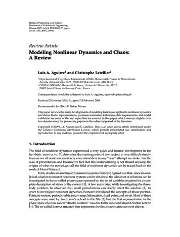
10CHAPTER 1. DYNAMICAL SYSTEMSFigure 1.3: Flow diagram for the logistic equation.1.2.2Logistic equationThis model for population growth was first proposed by Verhulst in 1838. Let N denotethe population in question. The dynamics are modeled by the first order ODE, N dN,(1.23) rN 1 dtKwhere N , r, and K are all positive. For N K the growth rate is r, but as N increases aquadratic nonlinearity kicks in and the rate vanishes for N K and is negative for N K.The nonlinearity models the effects of competition between the organisms for food, shelter,or other resources. Or maybe they crap all over each other and get sick. Whatever.There are two fixed points, one at N 0, which is unstable (f ′ (0) r 0). The other, atN K, is stable (f ′ (K) r). The equation is adimensionalized by defining ν N/Kand s rt, whenceν̇ ν(1 ν) .(1.24)Integrating, ν dν ds d lnν(1 ν)1 ν ν(s) ν0 ν0 1 ν0 exp( s).(1.25) As s , ν(s) 1 ν0 1 1 e s O(e 2s ), and the relaxation to equilibrium (ν 1)is exponential, as usual.Another application of this model is to a simple autocatalytic reaction, such asA X 2X ,(1.26)i.e. X catalyses the reaction A X. Assuming a fixed concentration of A, we haveẋ κ a x κ x2 ,(1.27)where x is the concentration of X, and κ are the forward and backward reaction rates.

1.2. N 1 SYSTEMS11αFigure 1.4: f (u) A u u , for α 1 and α 1.1.2.3Singular f (u)αSuppose that in the vicinity of a fixed point we have f (u) A u u , with A 0. Wenow analyze both sides of the fixed point.u u : Let ǫ u u. Thenǫ̇

S. Strogatz, Nonlinear Dynamics and Chaos (Addison-Wesley, 1994) S. Neil Rasband, Chaotic Dynamics of Nonlinear Systems (Wiley, 1990) J. Guckenheimer and P. Holmes, Nonlinear Oscillations, Dynamical Systems, and Bi-furcations of Vector Fields (Springer, 1983) E. A. Jackson, Perspectives of