WIXLIB

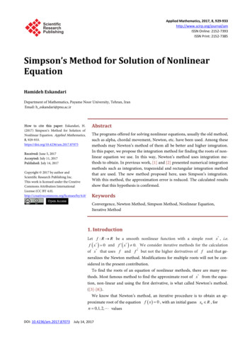
Note that sα 0 for α N1 . These dynamics arise from gradient descent on the energy function1 X1 X α β 2E (sα aα · bα )2 (a · b ) ,2τ α2τ(6)α6 βand display an interesting combination of cooperative and competitive interactions. Consider the first termsin each equation. In these terms, the connectivity modes from the two layers, aα and bα associated with thesame input-output mode of strength sα , cooperate with each other to drive each other to larger magnitudesas well as point in similar directions in the space of hidden units; in this fashion these terms drive theproduct of connectivity modes aα · bα to reflect the input-output mode strength sα . The second termsdescribe competition between the connectivity modes in the first (aα ) and second (bβ ) layers associated withdifferent input modes α and β. This yields a symmetric, pairwise repulsive force between all distinct pairs offirst and second layer connectivity modes, driving the network to a decoupled regime in which the differentconnectivity modes become orthogonal.1.2The final outcome of learningThe fixed point structure of gradient descent learning was worked out in [19]. In the language of the connectivity modes, a necessary condition for a fixed point is aα · bβ sα δαβ , while aα and bα are zero wheneversα 0. To satisfy these relations for undercomplete hidden layers (N2 N1 , N2 N3 ), aα and bα can be r31nonzero for at most N2 values of α. Since there are rank(Σ ) r nonzero values of sα , there areN2families of fixed points. However, all of these fixed points are unstable, except for the one in which only thefirst N2 strongest modes, i.e. aα and bα for α 1, . . . , N2 are active. Thus remarkably, the dynamics in (5)has only saddle points and no non-global local minima [19]. In terms of the original synaptic variables W 21and W 32 , all globally stable fixed points satisfyPN2W 32 W 21 α 1(7)sα uα vαT .Hence when learning has converged, the network will represent the closest rank N2 approximation to thetrue input-output correlation matrix. In this work, we are interested in understanding the dynamical weighttrajectories and learning time scales that lead to this final fixed point.1.3The time course of learning241.510.5bIt is difficult though to exactly solve (5) starting from arbitrary initialconditions because of the competitive interactions between differentinput-output modes. Therefore, to gain intuition for the general dynamics, we restrict our attention to a special class of initial conditionsof the form aα and bα rα for α 1, . . . , N2 , where rα · rβ δαβ ,with all other connectivity modes aα and bα set to zero (see [20] forsolutions to a partially overlapping but distinct set of initial conditions, further discussed in Supplementary Appendix A). Here rα isa fixed collection of N2 vectors that form an orthonormal basis forsynaptic connections from an input or output mode onto the set ofhidden units. Thus for this set of initial conditions, aα and bα pointin the same direction for each alpha and differ only in their scalarmagnitudes, and are orthogonal to all other connectivity modes. Suchan initialization can be obtained by computing the SVD of Σ31 andTtaking W 32 U 33 Da RT , W 21 RDb V 11 where Da , Db are diagonal, and R is an arbitrary orthogonal matrix; however, as we show0 0.5 1 1.5 2 2 10a12Figure 2: Vector field (blue), stablemanifold (red) and two solution trajectories (green) for the two dimensional dynamics of a and b in (8),with τ 1, s 1.

in subsequent experiments, the solutions we find are also excellentapproximations to trajectories from small random initial conditions.It is straightforward to verify that starting from these initial conditions, aα and bα will remain parallel to rαfor all future time. Furthermore, because the different active modes are orthogonal to each other, they do notcompete, or even interact with each other (all dot0.6products in the second terms of (5)-(6) are 0).LinearTanh)/t0.20.1half40200.40.3analy60 tanaly0.5(tmode strength80000500t (Epochs) 0.1100005101520Input output mode2530Figure 3: Left: Dynamics of learning in a three layer neural network. Curves show the strength of thenetwork’s representation of seven modes of the input-output correlation matrix over the course of learning.Red traces show analytical curves from Eqn. 12. Blue traces show simulation of full dynamics of a linearnetwork (Eqn. (2)) from small random initial conditions. Green traces show simulation of a nonlinearthree layer network with tanh activation functions. To generate mode strengths for the nonlinear network,we computed the nonlinear network’s evolving input-output correlation matrix, and plotted the diagonalTelements of U 33 Σ31 tanh V 11 over time. The training set consists of 32 orthogonal input patterns, eachassociated with a 1000-dimensional feature vector generated by a hierarchical diffusion process describedin [16] with a five level binary tree and flip probability of 0.1. Modes 1, 2, 3, 5, 12, 18, and 31 are plottedwith the rest excluded for clarity. Network training parameters were λ 0.5e 3 , N2 32, u0 1e 6 .Right: Delay in learning due to competitive dynamics and sigmoidal nonlinearities. Vertical axis shows thedifference between simulated time of half learning and the analytical time of half learning, as a fraction ofthe analytical time of half learning. Error bars show standard deviation from 100 simulations with randominitializations.Thus this class of conditions defines an invariant manifold in weight space where the modes evolve independently of each other.If we let a aα · rα , b bα · rα , and s sα , then the dynamics of the scalar projections (a, b) obeys,τda b (s ab),dtτdb a (s ab).dt(8)Thus our ability to decouple the connectivity modes yields a dramatically simplified two dimensional nonlinear system. These equations can by solved by noting that they arise from gradient descent on the error,E(a, b) 12τ (s ab)2 .(9)This implies that the product ab monotonically approaches the fixed point s from its initial value. Moreover,E(a, b) satisfies a symmetry under the one parameter family of scaling transformations a λa, b λb .This symmetry implies, through Noether’s theorem, the existence of a conserved quantity, namely a2 b2 ,which is a constant of motion. Thus the dynamics simply follows hyperbolas of constant a2 b2 in the (a, b)plane until it approaches the hyperbolic manifold of fixed points, ab s. The origin a 0, b 0 is also afixed point, but is unstable. Fig. 2 shows a typical phase portrait for these dynamics.As a measure of the timescale of learning, we are interested in how long it takes for ab to approach s fromany given initial condition. The case of unequal a and b is treated in the Supplementary Appendix A due tospace constraints. Here we pursue an explicit solution with the assumption that a b, a reasonable limit5

when starting with small random initial conditions. We can then track the dynamics of u ab, which from(8) obeysdτ u 2u(s u).(10)dtThis equation is separable and can be integrated to yieldZ ufduτuf (s u0 )t τ ln.(11)2u(s u)2su0 (s uf )u0Here t is the time it takes for u to travel from u0 to uf . If we assume a small initial condition u0 , andask when uf is within of the fixed point s, i.e. uf s , then the learning timescale in the limit 0is t τ /s ln (s/ ) O(τ /s) (with a weak logarithmic dependence on the cutoff). This yields a key result:the timescale of learning of each input-output mode α of the correlation matrix Σ31 is inversely proportionalto the correlation strength sα of the mode. Thus the stronger an input-output relationship, the quicker it islearned.We can also find the entire time course of learning by inverting (11) to obtainuf (t) se2st/τ. 1 s/u0(12)e2st/τThis time course describes the temporal evolution of the product of the magnitudes of all weights from aninput mode (with correlation strength s) into the hidden layers, and from the hidden layers to the same outputmode. If this product starts at a small value u0 s, then it displays a sigmoidal rise which asymptotesto s as t . This sigmoid can exhibit sharp transitions from a state of no learning to full learning.This analytical sigmoid learning curve is shown in Fig. 3 to yield a reasonable approximation to learningcurves in linear networks that start from random initial conditions that are not on the orthogonal, decoupledinvariant manifold–and that therefore exhibit competitive dynamics between connectivity modes–as well asin nonlinear networks solving the same task. We note that though the nonlinear networks behaved similarlyto the linear case for this particular task, this is likely to be problem dependent.2Deeper multilayer dynamicsThe network analyzed in Section 1 is the minimal example of a multilayer net, with just a single layer ofhidden units. How does gradient descent act in much deeper networks? We make an initial attempt in thisdirection based on initial conditions that yield particularly simple gradient descent dynamics.In a linear neural network with Nl layers and hence Nl 1 weight matrices indexed by W l , l 1, · · · , Nl 1,the gradient descent dynamics can be written as!T "!# l 1!TNYNYl 1l 1Yd lτ W WiΣ31 W i Σ11Wi,(13)dti 1i 1i l 1whereQbi aW i W b W (b 1) · · · W (a 1) W a with the caveat thatQbi aW i I, the identity, if a b.To describe the initial conditions, we suppose that there are Nl orthogonal matrices Rl that diagonalizeTthe starting weight matrices, that is, Rl 1Wl (0)Rl Dl for all l, with the caveat that R1 V 11 and33RNl U . This requirement essentially demands that the output singular vectors of layer l be the inputsingular vectors of the next layer l 1, so that a change in mode strength at any layer propagates to theoutput without mixing into other modes. We note that this formulation does not restrict hidden layer size;each hidden layer can be of a different size, and may be undercomplete or overcomplete. Making the6

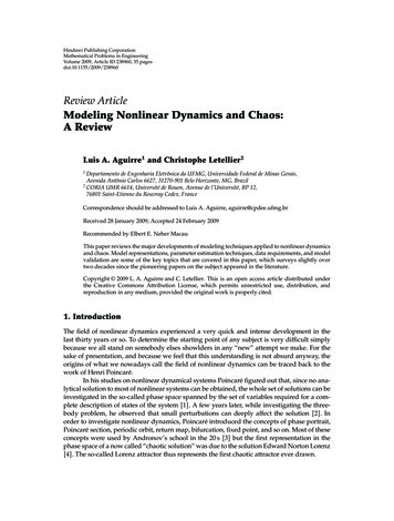
change of variables Wl Rl 1 W l RlT along with the assumption that Σ11 I leads to a set of decoupledconnectivity modes that evolve independently of each other. In analogy to the simplification occurring in thethree layer network from (2) to (8), each connectivity mode in the Nl layered network can be described byNl 1 scalars a1 , . . . , aNl 1 , whose dynamics obeys gradient descent on the energy function (the analog of(9)),!2NYl 11E(a1 , · · · , aNl 1 ) s ai .(14)2τi 1This dynamics also has a set of conserved quantities a2i a2j arising from the energetic symmetry w.r.t. theatransformation ai λai , aj λj , and hence can be solved exactly. We focus on the invariant submanifoldQNl 1in which ai (t 0) a0 for all i, and track the dynamics of u i 1ai , the overall strength of thismode, which obeys (i.e. the generalization of (10)),du (Nl 1)u2 2/(Nl 1) (s u).(15)dtThis can be integrated for any positive integer Nl , though the expression is complicated. Once the overallstrength increases sufficiently, learning explodes rapidly.τEqn. (15) lets us study the dynamics of learning as depth limits to infinity. In particular, as Nl wehave the dynamicsd(16)τ u Nl u2 (s u)dtwhich can be integrated to obtain τuf (u0 s)111t log .(17)Nl s2u0 (uf s)su0sufRemarkably this implies that, for a fixed learning rate, the learning time tends to zero as Nl goes to infinity.This result depends on the continuous time formulation, however. Any implementation will operate indiscrete time and must choose a finite learning rate that yields stable dynamics. An estimate of the optimallearning rate can be derived from the maximum eigenvalue of the Hessian over the region of interest. For linear networks with ai aj a, this optimal learning rate αopt decays with depth as O Nl1s2 forlarge Nl (see Supplementary Appendix B). Incorporating this dependence of the learning rate on depth, thelearning time as depth approaches infinity still surprisingly remains finite: with the optimal learning rate, thedifference between learning times for an Nl 3 network and an Nl network is t t3 O (s/ ) forsmall (see Supplementary Appendix B.1). 41.2Optimal learning rate250Learning time (Epochs)To verify these predictions,we trained deep linear networks on the MNIST datasetwith depths ranging fromNl 3 to Nl 100.We used hidden layers of size1000, and calculated the iteration at which training error fell below a fixed threshold corresponding to nearlycomplete learning. We optimized the learning rate separately for each depth by training each network with twenty200150100500050Nl (Number of layers)100x 1010.80.60.40.20050Nl (Number of layers)100Figure 4: Left: Learning time as a function of depth on MNIST. Right:Empirically optimal learning rates as a function of depth.7

rates logarithmically spacedbetween 10 4 and 10 7 and picking the fastest (see Supplementary Appendix C for details). Networkswere initialized with decoupled initial conditions and starting initial mode strength u0 0.001. Fig. 4shows the resulting learning times, which saturate, and the empirically optimal learning rates, which scalelike O(1/Nl ) as predicted.Thus learning times in deep linear networks that start with decoupled initial conditions are only a finiteamount slower than a shallow network regardless of depth. Moreover, the delay incurred by depth scalesinversely with the size of the initial strength of the association. Hence finding a way to initialize the modestrengths to large values is crucial for fast deep learning.3Finding good weight initializations: on greediness and randomnessThe previous subsection revealed the existence of a decoupled submanifold in weight space in which connectivity modes evolve independently of each other during learning, and learning times can be independentof depth, even for arbitrarily deep networks, as long as the initial composite, end to end mode strength,denoted by u above, of every connectivity mode is O(1). What numerical weight initilization procedurescan get us close to this weight manifold, so that we can exploit its rapid learning properties?A breakthrough in training deep neural networks started with the discovery that greedy layer-wise unsupervised pretraining could substantially speed up and improve the generalization performance of standardgradient descent [17, 18]. Unsupervised pretraining has been shown to speed the optimization of deepnetworks, and also to act as a special regularizer towards solutions with better generalization performance[18, 12, 13, 14]. At the same time, recent results have obtained excellent performance starting from carefullyscaled random initializations, though interestingly, pretrained initializations still exhibit faster convergence[21, 13, 22, 3, 4, 1, 23] (see Supplementary Appendix D for discussion). Here we examine analytically howunsupervised pretraining achieves an optimization advantage, at least in deep linear networks, by findingthe special class of orthogonalized, decoupled initial conditions in the previous section that allow for rapidsupervised deep learning, for input-output tasks with a certain precise structure. Subsequently, we analyzethe properties of random initilizations.We consider the effect of using autoencoders as the unsupervised pretraining module [18, 12], for which theinput-output correlation matrix Σ31 is simply the input correlation matrix Σ11 . Hence the SVD of Σ31 isPCA on the input correlation matrix, since Σ31 Σ11 QΛQT , where Q are eigenvectors of Σ11 and Λ isa diagonal matrix of variances. After pretraining, the weights thus converge to W 32 W 21 Σ31 (Σ31 ) 1 QQT . Recall that aα denotes the strength of mode α in W 21 , and bα denotes the strength in W 32 . If wefurther take the assumption that aα bα , as is typical when starting from small random weights, then theinput-to-hidden mapping will be W 21 R2 QT where R2 is an arbitrary orthogonal matrix. Now considerfine-tuning on a task with input-output correlations Σ31 U 33 S 31 V 11 . The pretrained initial conditionTW 21 R2 QT will be a decoupled initial condition for the task, W 21 R2 D1 V 11 , providedQ V 11 .(18)Hence we can state the underlying condition required for successful greedy pretraining in deep linear networks: the right singular vectors of the ultimate input-ouput task of interest V 11 must be similar to theprincipal components of the input data Q. This is a quantitatively precise instantiation of the intuitive ideathat unsupervised pretraining can help in a subsequent supervised learning task if (and only if) the statisticalstructure of the input is consistent with the structure of input-output map to be learned. Moreover, this quantitative instantiation of this intuitive idea gives a simple empirical criterion that can be evaluated on any newdataset: given the input-output correlation Σ31 and input correlation Σ11 , compute the right singular vectorsTV 11 of Σ31 and check that V 11 Σ11 V 11 is approximately diagonal. If the condition in Eqn. (18) holds,8

45x 103x 10100200 300Epoch400500Figure 5: MNIST satisfies the consistency condition for greedy pretraining. Left: Submatrix from the rawTMNIST input correlation matrix Σ11 . Center: Submatrix of V 11 Σ11 V 11 which is approximately diagonalas required. Right: Learning curves on MNIST for a five layer linear network starting from random (black)and pretrained (red) initial conditions. Pretrained curve starts with a delay due to pretraining time. The smallrandom initial conditions correspond to all weights chosen i.i.d. from a zero mean Gaussian with standarddeviation 0.01.autoencoder pretraining will have properly set up decoupled initial conditions for W 21 , with an appreciableinitial association strength near 1. This argument also goes through straightforwardly for layer-wise pretraining of deeper networks. Fig. 5 shows that this consistency condition empirically holds on MNIST, and thata pretrained deep linear neural network learns faster than one started from small random initial conditions,even accounting for pretraining time (see Supplementary Appendix E for experimental details).As an alternative to greedy layerwise pre-training, [13] proposed choosing appropriately scaled initial conditions on weights that would preserve the norm of typical error vectors as they were backpropagated throughthe deep network. In our context, the appropriate norm-preserving scaling for the initial condition of anN by N connectivity matrix W between any two layers corresponds to choosing each weight i.i.d. from azero mean Gaussian with standard deviation 1/ N . With this choice, hv T W T W viW v T v, where h·iWdenotes an average over distribution of the random matrix W . Moreover, the distribution of v T W T W v concentrates about its mean for large N . Thus with this scaling, in linear networks, both the forward propagationof activity, and backpropagation of gradients is typically norm-preserving. However, with this initialization,the learning time with depth on linear networks trained on MNIST grows with depth (Fig. 6A, left, blue).This growth is in distinct contradiction with the theoretical prediction, made above, of depth independentlearning times starting from the decoupled submanifold of weights with composite mode strength O(1).This suggests that the scaled random initialization scheme, despite its norm-preserving nature, does not findthis submanifold in weight space. In contrast, learning times with greedy layerwise pre-training do not growwith

solutions of learning dynamics in deep linear networks to numerical simulations of learning dynamics in deep non-linear networks, and find that our analytical solutions provide a reasonable approximation. Our solutions also reflect nonlinear phenomena seen in simulations, including alte