Transcription
Synchronous Machine ModelingNovember 21, 2019WECC MVWGJamie Weber, Ph.D.Director of Software Developmentweber@powerworld.com
Synchronous Machine Modeling Electric machines are used to convert mechanicalenergy into electrical energy (generators) and fromelectrical energy into mechanical energy (motors)– Many devices can operate in either mode, but areusually customized for one or the other Vast majority of electricity is generated usingsynchronous generators and some is consumedusing synchronous motors, so we'll start there– Don’t worry: We’ll talk about wind and solar later! There is much literature on subject, and sometimesit is overly confusing with the use of differentconventions and nomenclature1
Transient Stability Modeling A good comprehensive book on this typeof analysis is the by Prabha Kundur and iscalled Power System Stability and Controlpublished in 1994– Book is too detailed for a classroomtextbook, but it is a really great as areference book once you’re working Another good theoretical book is PowerSystem Dynamics and Stability by PeterSauer and M.A. Pai from 1998.– The derivation in this book of thesynchronous machine equations veryclosely matches the equations andnomenclature used in commercial softwaretools2
Synchronous MachineTerminology Positional Winding Terms– Stator (Stationary portion of generator)– Rotor (Rotating portion of generator) Functional Winding Terms– Armature Winding (three-phase AC winding that carries the power) Normally this is on the Stator– Field Winding (DC current winding) Normally this is on the Rotor– Amortisseur Winding (or Damper winding) An extra winding that provides start-up torque and damping Basically a winding that creates a force that attempts to bring machine tosynchronous speed (60 Hz)– Armature Poles Following slide shows two dots for each (A, B, C) phase one “in” and one “out” This represents a 2 pole machine If you just repeated this 4 additional times for each phase then you’d have an “8pole” machine More poles means the machine doesn’t need to spin as fast to create 60 Hz3
Modeling the Generator Rotor d Direct Axis– Spinning axis directly inline with the “North Pole”of the field winding q Quadrature Axis– Spinning axis 90degrees out ofAir Gapphase with thedirect axis– (We choose Leading) Field Rotor Angle (𝛿)– Angle betweenq-axis andPhase A axis– (this is arbitrary)WindingArmatureWindingRight-Hand rule defines axes ofphase a, b, and c as well as direct axis4
Careful of Conventions whenlooking at Textbooks!Software Convention Choice q-axis leads the d-Axis Rotor angle w.r.t. to q-axis(Also Sauer/Pai book)Kundar BookRotor angle withrespect to d-axisAnderson/Fouad BookRotor angle withrespect to d-axisq-axis lags insteadof leads5
Synchronous Machine Basics of Synchronous Machine Model– Exciter applies DC current to rotor making it an electromagnet– Turbine/Governor spins rotor– Spinning magnet creates AC powerTurbine/GovernorCreates amechanicaltorque to spin therotorExciterCreates a DCvoltage to apply toRotor Winding,resulting in anelectromagnet6
Two Main Types of SynchronousMachines Round Rotor– Air-gap is constant, used withhigher speed machines Salient Rotor (often called SalientPole)– Air-gap varies circumferentially– Used with many pole, slowermachines such as hydro– Narrowest part of gap in the d-axisand the widest along the /synchronous-machine-rotor-7
Synchronous Machine StatorImage Source: Glover/Overbye/Sarma Book, Sixth Edition, Beginning of Chapter 8 Photo8
Synchronous Machine Rotors Rotors are essentially electromagnetsTwo pole (P)round rotorSix pole salientrotorImage Source: Dr. Gleb Tcheslavski, ee.lamar.edu/gleb/teaching.htm9
Synchronous Machine RotorHigh polesalientrotorShaftPart of exciter,which is usedto control thefield currentImage Source: Dr. Gleb Tcheslavski, ee.lamar.edu/gleb/teaching.htm10
Synchronous Machine Modeling:Sauer/Pai Book Good Reference Stator/Armature Windings– 3 bal. windings (a,b,c) Rotor/Field winding– Field windingconnected to Exciter (fd)– “d” axis damper (1d)– 2 “q” axis dampers (1q, 2q) “Damper” windings do nothave external connections– They stabilize the electricaloperation of the machine– Also provide start-up torquefor the machine11
Dynamic Equations of aSynchronous Machine Start with Newton’s second law Force Mass * Acceleration 𝐹 𝑀𝑑𝑣𝑑𝑡and𝑑𝑥𝑑𝑡 𝑣 We have a rotational system though, so instead weend up with something a little different Torque Moment of Inertia * Angular Acceleration 𝑇 𝐽𝑑𝜔𝑑𝑡and𝑑𝛿𝑑𝑡 𝜔 Electrical Equations just apply the same equationsto the circuits for the 7 windings a, b, c, fd, 1d, 1q,2q 𝑣 𝑖𝑟 𝑑𝜆𝑑𝑡12
Fundamental Laws Kirchhoff’s Voltage Law, Ohm’s Law, Faraday’sLaw, Newton’s Second LawStator𝑑𝜆𝑎𝑣𝑎 𝑖𝑎 𝑟𝑠 𝑑𝑡𝑑𝜆𝑏𝑣𝑏 𝑖𝑏 𝑟𝑠 𝑑𝑡𝑑𝜆𝑐𝑣𝑐 𝑖𝑐 𝑟𝑠 𝑑𝑡Rotor𝑑𝜆𝑓𝑑𝑑𝑡𝑑𝜆1𝑑 𝑖1𝑑 𝑟1𝑑 𝑑𝑡𝑑𝜆1𝑞 𝑖1𝑞 𝑟1𝑞 𝑑𝑡𝑑𝜆2𝑞 𝑖2𝑞 𝑟2𝑞 𝑑𝑡𝑣𝑓𝑑 𝑖𝑓𝑑 𝑟𝑓𝑑 𝑣1𝑑𝑣1𝑞𝑣2𝑞Shaft𝑑𝜃shaft 2 𝜔𝑑𝑡𝑃2 𝑑𝜔𝐽 𝑇𝑚 𝑇𝑒 𝑇𝑓𝜔𝑃 𝑑𝑡13
Deriving Equations for Rotor Algebra and trigonometry end up beingextremely complex– Results give inductances between phases that area function of the cosine of rotor angle. Yuck!– Special transformations are done to transform theabc phase quantities into another reference frame Called the dq0 transformation– Might hear it called “Park’s Transformation” after Robert H.Park who introduced this concept in 1929 (his was slightlyscaled transformation, but was the same idea) Parks’ 1929 paper voted 2nd most important powerpaper of 20th century (1st was Fortescue’s sym.components) Convention used here is the q-axis leads the d-axis(which is the IEEE standard)14
dq0 Transformation This is a very similar idea as symmetrical components when discussing faultanalysis (different matrix conversion though)We can say thanks to engineers who figured this all out for us 80 years ago!We end up with 14 equations that go through conversion similar to followingAlso make some more “magic” per unit choices to make things clean-up moredq015
Dq0 Transformations vd va vq Tdqo vb v vc o vd va v T 1 v b dqo q v vc o or i, In the next few slideswe’ll quickly gothrough how thesebasic equations aretransformed into thestandard machinemodels. The pointis to show the physicalbasis for the models.And there is NO quizat the end!!16
dq0 TransformationsTdqo P sin 2 shaft 2 P cos shaft32 1 2 2 2 P Psin shaft sin shaft 3 3 2 2 2 2 P Pcos shaft cos shaft 233 2 11 22 with the inverse,Note that thetransformation depends on the1 shaft angle. PPsin cos shaftshaft 22 P2 P2 1Tdqo sin shaft cos shaft 1 3 3 2 22 2 P P sin cos shaft 1 2 shaft 3 3 217
Transformed SystemStatord vd rsid q ddtd qvq rsiq d dtd vo rsio odtRotorv fd r fd i fd Shaftd fddtd 1dv1d r1d i1d dtd 1qv1q r1qi1q dtd 2 qv2 q r2 qi2 q dtd shaft 2 Pdt2 d J Tm Te T f P dtConverted from abc reference frame to the dq0reference frameExtra Terms show up due to transformation18
Electrical & MechanicalRelationshipsd Electrical system:v iR dt(voltage)d vi i R i(power)dtMechanical system: 2 d P is the number ofJ Tm Te T fw (torque)poles (e.g. 2,4,6) P dt222 2 d 2J Tm Te T fwdt PPP P 2MechanicalPowerElectrical Torque(power)Friction andWindage19
Electric Torque Derivation Friction and Windage Torque: we ignore Mechanical Torque: this is an input to thesystem Electrical Torque– Torque is derived by looking at the overall energybalance in the system– Three systems: electrical, mechanical and thecoupling magnetic field Electrical system losses are in the form of resistance Mechanical system losses are in the form of friction– Coupling field is assumed to be lossless, hence wecan track how energy moves between theelectrical and mechanical systems20
Energy ConversionNo Losses in theCoupling Field21
Skip the Derivation A lot of interesting calculus and algebra usingthe “Conservative Coupling Field” assumptiongive us the electrical torque𝑇𝑒𝑙𝑒𝑐3𝑃 𝜆𝑑 𝐼𝑞 𝜆𝑞 𝐼𝑑22 Also we define where 𝜔𝑠 is the synchronousspeedP shaft st2 This makes our mechanical equationsd sdt2 d 3 P J Tm d iq qid T f p dt 2 2 ()22
Generator Swing Equation Anyway, after a lot of additional algebra, software tools model theswing equations as follows with values in per unit– 2𝐻𝑑𝜔𝑑t 𝑃𝑚𝑒𝑐ℎ1 𝜔 𝑇𝑒𝑙𝑒𝑐and𝑑𝛿𝑑𝑡 𝜔 If you use a more complete model of the rotor of a generator, thenthe 𝑇𝑒𝑙𝑒𝑐 term has some inherent damping in it In academic settings, as we’ll introduce in a moment, the rotormodeling has no inherent damping in it (which makes your resultsreally oscillate)– To overcome this, folks in the 1960s added an extra 𝐷𝜔 term as follows𝑑𝜔 𝑃𝑚𝑒𝑐ℎ 𝐷𝜔2𝐻 𝑇𝑒𝑙𝑒𝑐𝑑𝑡1 𝜔– This term should NOT be used to model the damping in the moreaccurate rotor models such as GENROU, GENSAL, GENTPF, GENTPJ, etc.– Friction and Windage term has been removed for our purposes23
From here Lots of Per-UnitChoices Pages 30 – 42 in the Sauer/Pai textbook gothrough a ton of per unit scaling and lots ofalgebra Small notation differences, but we end upwith the equations on the next page whichlargely match what Sauer/Pai derive– Different Notation though (Our notation Sauer/Pai) ′d 1𝑑 ′𝑞 2𝑞OurNotationSauer/PaiNotation24
Variables and Constants Per Unit Model Variables– 𝜔𝑠 is the synchronous speed (2 60)– 𝜔𝑝𝑢 is the deviation of rotor speed away from synchronousspeed– 𝐼𝑑 , 𝐼𝑞 , 𝐼0 are the stator current in dq0 reference– 𝑉𝑑𝑡𝑒𝑟𝑚 , 𝑉𝑞𝑡𝑒𝑟𝑚 , 𝑉0𝑡𝑒𝑟𝑚 are the stator voltage in dq0 reference– 𝑑 , 𝑞 , 0 are the stator flux in the dq0 reference– 𝐸𝑑′ , 𝐸𝑞′ , ′𝑞 , and ′𝑑 represent per-unitized versions of the rotorfluxes– 𝐸𝑓𝑑 is the field voltage input (from exciter)– 𝑃𝑚𝑒𝑐ℎ is the mechanical power input (from turbine/governor) Per Unit Model Constants′′′′′′– 𝐻, 𝐷, 𝑅𝑠 , 𝑋𝑑 , 𝑋𝑑′ , 𝑋𝑑′′ , 𝑋𝑞 , 𝑋𝑞′ , 𝑋𝑞′′ , 𝑋𝑙 , 𝑇𝑑𝑜, 𝑇𝑑𝑜, 𝑇𝑞𝑜, 𝑇𝑞𝑜25
Final Complete Model ofPer-Unitized Equations2 Mechanical Dynamic Equations𝑑δdtAlgebraic Relationship between Stator andRotor Fluxes 𝜔𝑝𝑢 𝜔𝑠2𝐻d𝜔𝑑𝑡 𝑃𝑚𝑒𝑐ℎ 𝐷𝜔1 𝜔𝑝𝑢 𝑑 𝐼𝑑 𝑋𝑑′′ 𝐸𝑞′ 𝑑 𝐼𝑞 𝑞 𝐼𝑑3 Stator Dynamic Equations1 𝑑 𝑑 𝑅𝑠 𝐼𝑑 1 𝜔𝑝𝑢 𝑞 𝑉𝑑𝑡𝑒𝑟𝑚𝜔𝑠 𝑑𝑡1 𝑑 𝑞 𝑅𝑠 𝐼𝑞 1 𝜔𝑝𝑢 𝑑 𝑉𝑞𝑡𝑒𝑟𝑚𝜔𝑠 𝑑𝑡1 𝑑 0 𝑅𝑠 𝐼0 𝑉0𝑡𝑒𝑟𝑚 𝑞 𝐼𝑞 𝑋𝑞′′ 𝑋𝑑′′ 𝑋𝑙𝑋𝑑′ 𝑋𝑙′′′ 𝑋𝑞 𝑋𝑙𝐸𝑑 ′𝑋𝑞 𝑋𝑙 ′𝑑 𝑋𝑑′ 𝑋𝑑′′𝑋𝑑′ 𝑋𝑙′′′′ 𝑋𝑞 𝑋𝑞 𝑞 ′𝑋𝑞 𝑋𝑙The 3 stator equations define whatare known as the stator transients.𝜔𝑠 𝑑𝑡4 Rotor Dynamic Equations′𝑇𝑑𝑜d𝐸𝑞′dt′′ d𝐸𝑑𝑇𝑞𝑜dt′′𝑇𝑑𝑜𝑑 ′ddt′d 𝑞′′𝑇𝑞𝑜dt 𝐸𝑓𝑑 𝐸𝑞′ 𝑋𝑑 𝑋𝑑′ 𝐸𝑑′ 𝑋𝑞 𝑋𝑞′𝐼𝑑 𝐼𝑞 𝑋𝑑′ 𝑋𝑑′′2𝑋𝑑′ 𝑋𝑙𝑋𝑞′ 𝑋𝑞′′2𝑋𝑞′ 𝑋𝑙 ′𝑑 𝑋𝑑′ 𝑋𝑙 𝐼𝑑 𝐸𝑞′ ′𝑞 𝑋𝑞′ 𝑋𝑙 𝐼𝑞 𝐸𝑑′′ 𝑑 𝑋𝑑′ 𝑋𝑙 𝐼𝑑 𝐸𝑞′ ′𝑞 𝑋𝑞′ 𝑋𝑙 𝐼𝑞 𝐸𝑑′26
Stator Flux Differential Equations Stator Differential Equations1 𝑑 𝑑𝜔𝑠 𝑑𝑡1 𝑑 𝑞𝜔𝑠 𝑑𝑡1 𝑑 0𝜔𝑠 𝑑𝑡 𝑅𝑠 𝐼𝑑 1 𝜔𝑝𝑢 𝑞 𝑉𝑑𝑡𝑒𝑟𝑚 𝑅𝑠 𝐼𝑞 1 𝜔𝑝𝑢 𝑑 𝑉𝑞𝑡𝑒𝑟𝑚 𝑅𝑠 𝐼0 𝑉0𝑡𝑒𝑟𝑚 These have a time constant that is11 0.00265𝜔𝑠 2𝜋60– This is about 1/6th of a cycle and is MUCH faster thanthe phenomena that transient stability is concernedwith Transient Stability Simulations neglect these27
Impact on StudiesStator transients are not usually consideredin transient stability studiesImage Source: P. Kundur, Power System Stability and Control, EPRI, McGraw-Hill, 199428
Elimination of Stator Transients Mathematics is kind of neat and you get to useterms like “Integral Manifold” and sound reallysmart Easier way to think of it– Regardless of what the derivative of these fluxes are,1they are multiplied by a very small numberand𝜔𝑠thus the left-hand side is near zero anyway, soapproximation is made1 𝑑 𝑑 0 𝑅𝑠 𝐼𝑑 1 𝜔𝑝𝑢 𝑞 𝑉𝑑𝑡𝑒𝑟𝑚𝜔𝑠 𝑑𝑡1 𝑑 𝑞 0 𝑅𝑠 𝐼𝑞 1 𝜔𝑝𝑢 𝑑 𝑉𝑞𝑡𝑒𝑟𝑚𝜔𝑠 𝑑𝑡1 𝑑 0 0 𝑅𝑠 𝐼0 𝑉0𝑡𝑒𝑟𝑚𝜔𝑠 𝑑𝑡29
Stator Equations BecomesAlgebraic Network Equation This gives us the followingAlso remember stator flux relationships 𝑑 𝑉𝑑𝑡𝑒𝑟𝑚 𝑅𝑠 𝐼𝑑 1 𝜔𝑝𝑢 𝑞𝑉𝑞𝑡𝑒𝑟𝑚 𝑅𝑠 𝐼𝑞 1 𝜔𝑝𝑢 𝑑 𝑞 ′′′′′′ 𝑋𝑑 𝑋𝑑′ 𝑋𝑑 𝑋𝑙 𝐸𝑞 ′ 𝑑 ′𝑋𝑑 𝑋𝑙𝑋𝑑 𝑋𝑙′′𝑋𝑞 𝑋𝑙𝑋𝑞′ 𝑋𝑞′′ 𝐼𝑞 𝑋𝑞′′ 𝐸𝑑′ ′ ′𝑞 ′𝑋 𝑋𝑋 𝑋 𝐼𝑑 𝑋𝑑′′𝑞𝑙𝑞𝑙 Take the algebraic flux relationship and plug it in𝑉𝑑𝑡𝑒𝑟𝑚 𝑅𝑠 𝐼𝑑 1 𝜔𝑝𝑢 𝐼𝑞 𝑋𝑞′′′′′ 𝑋𝑞 𝑋𝑙 𝐸𝑑 𝑋 ′ 𝑋𝑙𝑞𝑉𝑞𝑡𝑒𝑟𝑚 𝑅𝑠 𝐼𝑞 1 𝜔𝑝𝑢 𝐼𝑑 𝑋𝑑′′𝑋𝑑′′ 𝑋𝑙′𝐸𝑞 𝑋 ′ 𝑋𝑙𝑑 𝑋𝑞′ 𝑋𝑞′′′ 𝑞 𝑋 ′ 𝑋𝑙𝑞 ′′′′ 𝑋𝑑 𝑋𝑑 𝑑 𝑋 ′ 𝑋𝑙𝑑 Group Terms𝑉𝑑𝑡𝑒𝑟𝑚 𝑅𝑠 𝐼𝑑 1 𝜔𝑝𝑢 𝑋𝑞′′ 𝐼𝑞𝑉𝑞𝑡𝑒𝑟𝑚 𝑅𝑠 𝐼𝑞 1 𝜔𝑝𝑢 𝑋𝑑′′ 𝐼𝑑 1 𝜔𝑝𝑢′′′ 𝑋𝑞 𝑋𝑙 𝐸𝑑 𝑋 ′ 𝑋𝑙𝑞 1 𝜔𝑝𝑢′′′ 𝑋𝑑 𝑋𝑙 𝐸𝑞 𝑋 ′ 𝑋𝑙𝑑 ′′′′ 𝑋𝑞 𝑋𝑞 𝑞 𝑋 ′ 𝑋𝑙𝑞 ′′′′ 𝑋𝑑 𝑋𝑑 𝑑 𝑋 ′ 𝑋𝑙𝑑30
Stator Equation BecomesNetwork Equation Now define𝐸𝑑′′𝐸𝑞′′ ′′′ 𝑋𝑞 𝑋𝑙 𝐸𝑑 𝑋 ′ 𝑋𝑙𝑞′′′′ 𝑋𝑞 𝑋𝑞 𝑞 𝑋 ′ 𝑋𝑙𝑞 ′′′ 𝑋𝑑 𝑋𝑙 𝐸𝑞 𝑋 ′ 𝑋𝑙𝑑′′′′ 𝑋𝑑 𝑋𝑑 𝑑 𝑋 ′ 𝑋𝑙𝑑 This gives us the following𝑉𝑑𝑡𝑒𝑟𝑚 𝑅𝑠 𝐼𝑑 1 𝜔𝑝𝑢 𝑋𝑑′′ 𝐼𝑞 𝐸𝑑′′ 1 𝜔𝑝𝑢𝑉𝑞𝑡𝑒𝑟𝑚 𝑅𝑠 𝐼𝑞 1 𝜔𝑝𝑢 𝑋𝑑′′ 𝐼𝑑 𝐸𝑞′′ 1 𝜔𝑝𝑢 Consider term 1 𝜔𝑝𝑢 that remains– Similar to multiplying all the transmission line X values by per unitfrequency to scale the network impedances as system frequencychanges No one does this in transient stability, so we just remove the purple We leave the scaling of the internal voltage though𝑉𝑑𝑡𝑒𝑟𝑚 𝐸𝑑′′ 1 𝜔𝑝𝑢 𝑅𝑠 𝐼𝑑 𝑋𝑞′′ 𝐼𝑞𝑉𝑞𝑡𝑒𝑟𝑚 𝐸𝑞′′ 1 𝜔𝑝𝑢 𝑅𝑠 𝐼𝑞 𝑋𝑑′′ 𝐼𝑑31
Final Complete Model ofPer-Unitized EquationsAlgebraic Relationships𝐸𝑑′′ 𝐸𝑞′′ ′′′ 𝑋𝑞 𝑋𝑙 𝐸𝑑 ′ ′𝑞𝑋𝑞 𝑋𝑙′′′ 𝑋𝑑 𝑋𝑙 𝐸𝑞 ′ ′𝑑𝑋 𝑋𝑙𝑑𝑋𝑞′ 𝑋𝑞′′𝑋𝑞′ 𝑋𝑙𝑋𝑑′ 𝑋𝑑′′𝑋𝑑′ 𝑋𝑙 𝑑 𝐼𝑑 𝑋𝑑′′ 𝐸𝑞′′ 𝑞 𝐼𝑞 𝑋𝑑′′ 𝐸𝑑′′𝑉𝑑𝑡𝑒𝑟𝑚 𝐸𝑑′′ 1 𝜔𝑝𝑢 𝑅𝑠 𝐼𝑑 𝑋𝑞′′ 𝐼𝑞𝑉𝑞𝑡𝑒𝑟𝑚 𝐸𝑞′′ 1 𝜔𝑝𝑢 𝑅𝑠 𝐼𝑞 𝑋𝑑′′ 𝐼𝑑6 Differential ��𝑞𝑜5.6. 𝜔𝑝𝑢 𝜔𝑠d𝜔𝑑𝑡 d𝐸𝑞′dtd𝐸𝑑′dt𝑃𝑚𝑒𝑐ℎ 𝐷𝜔1 𝜔𝑝𝑢 𝑑 𝐼𝑞 𝑞 𝐼𝑑 𝐸𝑓𝑑 𝐸𝑞′ 𝑋𝑑 𝑋𝑑′𝐼𝑑 𝐸𝑑′ 𝑋𝑞 𝑋𝑞′𝐼𝑞 ′′′′ 𝑑 d𝑇𝑑𝑜 𝑑 dt′d 𝑞′′𝑇𝑞𝑜 ′𝑞 dt𝑋𝑑′ 𝑋𝑑′′2𝑋𝑑′ 𝑋𝑙𝑋𝑞′ 𝑋𝑞′′2𝑋𝑞′ 𝑋𝑙 ′𝑑 𝑋𝑑′ 𝑋𝑙 𝐼𝑑 𝐸𝑞′ ′𝑞 𝑋𝑞′ 𝑋𝑙 𝐼𝑞 𝐸𝑑′𝑋𝑑′ 𝑋𝑙 𝐼𝑑 𝐸𝑞′𝑋𝑞′ 𝑋𝑙 𝐼𝑞 𝐸𝑑′32
Field Voltage and Current Field Voltage (𝐸𝑓𝑑 ) is an input from the exciter The field current, 𝐼𝑓𝑑 , is defined in steady-state as𝐼𝑓𝑑 𝐸𝑓𝑑 /𝑋𝑚𝑑 Traditional, when we talk about a “field current” weare actually mean the product of the field currentand the mutual inductance 𝐼𝑓𝑑 𝑋𝑚𝑑 (also written𝐼𝑓𝑑 𝐿𝑎𝑑 )𝐿𝑎𝑑 𝐼𝑓𝑑 ′′ d𝐸𝑞𝑇𝑑𝑜dt𝐸𝑞′ 𝑋𝑑 𝑋𝑑′𝐼𝑑 𝑋𝑑′ 𝑋𝑑′′𝑋𝑑′ 𝑋𝑙2 ′𝑑 𝑋𝑑′ 𝑋𝑙 𝐼𝑑 𝐸𝑞′ 𝐸𝑓𝑑 𝐿𝑎𝑑 𝐼𝑓𝑑33
Multiple Machines This math is all very beautiful, but it is allrelated to a single machine that isconnected to a three-phase system We need a similar conversion for the abcquantities at all the network buses This requires us to do some more beautifulmath We will first convert all network abcquantities to a common reference framewe call the Synchronous Reference Frame34
Synchronously RotatingReference Frame That conversion is chosen as follows– It was chosen because the math works out so nicelycos 𝜔𝑡𝑇𝑠𝑦𝑛𝑐 23 sin 𝜔𝑡1/22𝜋32𝜋 sin 𝜔𝑡 31/2cos 𝜔𝑡 2𝜋32𝜋 sin 𝜔𝑡 31/2cos 𝜔𝑡 𝑣𝐷𝑉𝑎𝑣𝑄 𝑇𝑠𝑦𝑛𝑐 𝑉𝑏𝑣𝑂𝑉𝑐 Assume you have a 3-phase balanced voltagecos 𝜔𝑡𝑣𝐷2𝑣𝑄 3 sin 𝜔𝑡𝑣𝑂1/22𝜋32𝜋 sin 𝜔𝑡 31/2cos 𝜔𝑡 2𝜋32𝜋 sin 𝜔𝑡 31/2cos 𝜔𝑡 𝑉𝑡 cos 𝜔𝑡 𝛼2𝜋32𝜋𝑉𝑡 cos 𝜔𝑡 𝛼 3𝑉𝑡 cos 𝜔𝑡 𝛼 35
Synchronous Reference Framefor 3-Phase Balanced Operation Now multiply these out𝑣𝑑 𝑉𝑡𝑣𝑞 𝑉𝑡𝑣0 𝑉𝑡232 cos 𝜔𝑡 cos 𝜔𝑡 𝛼 cos 𝜔𝑡 sin 𝜔𝑡 cos 𝜔𝑡 𝛼 sin 𝜔𝑡 32 13 212𝜋23cos 𝜔𝑡 𝛼 cos 𝜔𝑡 𝛼 2𝜋32𝜋3cos 𝜔𝑡 𝛼 cos 𝜔𝑡 𝛼 2𝜋32𝜋132𝜋23 cos 𝜔𝑡 𝛼 cos 𝜔𝑡 sin 𝜔𝑡 2𝜋32𝜋3cos 𝜔𝑡 𝛼 cos 𝜔𝑡 𝛼 2𝜋32𝜋3 The 𝑣0 value will evaluation to 0.0– Three cosine waves shifted by2𝜋3sum to 0.0 Then use of the following trigonometry2𝜋2𝜋3133cos 𝑦 sin 𝑥 sin 𝑦 cos 𝑥 cos 𝑦 sin 𝑥 cos 𝑦 cos 𝑥 sin 𝑦3344442𝜋2𝜋3133cos 𝑥 cos 𝑦 sin 𝑥 sin 𝑦 cos 𝑥 cos 𝑦 sin 𝑥 cos 𝑦 cos 𝑥 sin 𝑦334444cos 𝑥 sin 𝑥 2𝜋2𝜋3313cos 𝑦 sin 𝑥 sin 𝑦 cos 𝑥 cos 𝑦 sin 𝑥 cos 𝑦 cos 𝑥 sin 𝑦334444sin 𝑥 2𝜋2𝜋3313cos 𝑦 sin 𝑥 sin 𝑦 cos 𝑥 cos 𝑦 sin 𝑥 cos 𝑦 cos 𝑥 sin 𝑦33444436
Synchronous Reference Framefor 3-Phase Balanced Operation Lots of terms cancel and you end up with232𝑉𝑡3𝑣𝑑 𝑉𝑡𝑣𝑞 323 sin2323cos2 cos 𝜔𝑡 cos 𝜔𝑡 𝛼 sin 𝜔𝑡 sin 𝜔𝑡 𝛼𝜔𝑡 cos 𝜔𝑡 𝛼 𝜔𝑡 sin 𝜔𝑡 𝛼𝑣0 0 The 2/3 and 3/2 terms cancel out and you get𝑣𝑑 𝑉𝑡 cos 𝜔𝑡 cos 𝜔𝑡 𝛼 sin 𝜔𝑡 sin 𝜔𝑡 𝛼𝑣𝑞 𝑉𝑡 sin 𝜔𝑡 cos 𝜔𝑡 𝛼 cos 𝜔𝑡 sin 𝜔𝑡 𝛼𝑣0 0 More Trigonometry and it simplifies to𝑣𝑑 𝑉𝑡 cos 𝛼𝑣𝑞 𝑉𝑡 sin 𝛼𝑣0 0All the 𝜔𝑡 termscancel out!37
Synchronous Reference Framefor 3-Phase Balanced Operation A-phase sinusoidal is 𝑉𝑡 cos 𝜔𝑡 𝛼– Magnitude of 𝑉𝑡 and phase difference from the“synchronous reference frame” of 𝛼 Value converted to the 𝑣𝐷 𝑉𝑡 cos 𝛼synchronous reference 𝑣𝑄 𝑉𝑡 sin 𝛼𝑣𝑂frame are0 That means we can treat this like a complexnumber and just jump right to𝑣𝐷 𝑗𝑣𝑄 𝑉𝑡 cos 𝛼 𝑗𝑉𝑡 sin 𝛼 𝑉𝑡 𝑒 𝑗𝛼 This is exactly what we always do in steadystate power flow equations, so this is nothingnew!38
Must Apply Same SynchronousReference Frame to Machine Remember that the abc quantities are converted tothe machine reference frame. We then need to additionally transform those tothe Network Reference𝑉𝑑𝑖𝑉𝑎 1𝑉𝑞𝑖𝑉𝑏 ���𝑖𝑉𝑎 1𝑣𝑄 𝑇𝑠𝑦𝑛𝑐 𝑉𝑏 𝑇𝑠𝑦𝑛𝑐 ��0𝑖 Need the matrix in yellow for direct conversion “Synchronous Reference Frame" Just call it the “Network Reference”– Network Reference Frame– Machine Reference Frame𝑣𝐷𝑉𝑑𝑖 1𝑣𝑄 𝑇𝑠𝑦𝑛𝑐 9
Converting Machine to NetworkReference Frame Remember how we converted the abc phase statorquantities to the dq0 reference frame PPcos shaft1 sin 2 shaft2 P2 P2 1Tdqo sin shaft cos shaft 1 3 3 2 22 2 P P sin cos shaft 1 2 shaft 3 3 2 Also remember our choice ofP shaft st2𝑃 Thus 𝜃𝑠ℎ𝑎𝑓𝑡 𝜔𝑠 𝑡 𝛿240
Converting Machine to NetworkReference Frame This makes our transformation matrix for aparticular machine “i” the followingsin 𝜔𝑡 𝛿 1𝑇𝑑𝑞0𝑖cos 𝜔𝑡 𝛿2𝜋sin 𝜔𝑡 𝛿 3 2𝜋sin 𝜔𝑡 𝛿 312𝜋cos 𝜔𝑡 𝛿 32𝜋cos 𝜔𝑡 𝛿 311 This means for our machine reference frame tonetwork reference frame we need the followingcos 𝜔𝑡 1𝑇𝑠𝑦𝑛𝑐 𝑇𝑑𝑞0 cos 𝜔𝑡 2𝜋23 sin 𝜔𝑡1/2 sin 𝜔𝑡 1/232𝜋3cos 𝜔𝑡 2𝜋 sin 𝜔𝑡 1/232𝜋3sin 𝜔𝑡 𝛿sin 𝜔𝑡 𝛿 sin 𝜔𝑡 𝛿 cos 𝜔𝑡 𝛿2𝜋32𝜋3cos 𝜔𝑡 𝛿 cos 𝜔𝑡 𝛿 12𝜋32𝜋31141
Converting Machine to NetworkReference Frame 1𝑇𝑠𝑦𝑛𝑐 𝑇𝑑𝑞0 2𝜋cos 𝜔𝑡cos 𝜔𝑡 sin 𝜔𝑡 sin 𝜔𝑡 231/2cos 𝜔𝑡 32𝜋2𝜋 sin 𝜔𝑡 31/232𝜋31/2sin 𝜔𝑡 𝛿sin 𝜔𝑡 𝛿 sin 𝜔𝑡 𝛿 cos 𝜔𝑡 𝛿2𝜋32𝜋3cos 𝜔𝑡 𝛿 cos 𝜔𝑡 𝛿 12𝜋32𝜋311 Use the trigonometry identities121 sin 𝛿21 cos 𝛿21 sin 𝛿2121 sin 2𝑥 𝛿21 cos 2𝑥 𝛿21 sin 2𝑥 𝛿2 sin 𝑥 sin 𝑥 𝛿 cos 𝛿 cos 2𝑥 𝛿 sin 𝑥 cos 𝑥 𝛿 cos 𝑥 cos 𝑥 𝛿 cos 𝑥 sin 𝑥 𝛿 When you group terms all the cos 2𝑥 𝛿and sin 2𝑥 𝛿 terms are going to cancel outand you only have the 1𝑇𝑠𝑦𝑛𝑐 𝑇𝑑𝑞0 32233 cos2323 sin2 sin 𝛿 cos 𝛿0𝛿𝛿0001All the 𝜔𝑡 termscancel out!42
Converting Machine to NetworkReference Frame Thus the conversion from Machine Network is 1𝑇𝑠𝑦𝑛𝑐 𝑇𝑑𝑞0 sin 𝛿 cos 𝛿0 cos 𝛿 sin 𝛿0001 And the conversion from Network Machine is 1𝑇𝑑𝑞0 𝑇𝑠𝑦𝑛𝑐 sin 𝛿 cos 𝛿0 cos 𝛿 sin 𝛿000143
Various Reference Conversions sin 𝛿 cos 𝛿 cos 𝛿 sin 𝛿00 1𝑇𝑠𝑦𝑛𝑐 𝑇𝑑𝑞0Machine (Rotor)Reference Frame 1𝑇𝑑𝑞0sin 𝜔𝑡 𝛿2𝜋32𝜋sin 𝜔𝑡 𝛿 3sin 𝜔𝑡 𝛿 cos 𝜔𝑡 𝛿2𝜋32𝜋cos 𝜔𝑡 𝛿 3cos 𝜔𝑡 𝛿 111ABC 𝑦𝑛𝑐cos 𝜔𝑡23 sin 𝜔𝑡1/22𝜋32𝜋 sin 𝜔𝑡 31/2cos 𝜔𝑡 2𝜋32𝜋 sin 𝜔𝑡 31/2cos 𝜔𝑡 44
We shall never speak of theABC Phase Reference Again! sin 𝛿 cos 𝛿 cos 𝛿 sin 𝛿00 1𝑇𝑠𝑦𝑛𝑐 𝑇𝑑𝑞0Machine (Rotor)Reference Frame 1𝑇𝑑𝑞0sin 𝜔𝑡 𝛿2𝜋32𝜋sin 𝜔𝑡 𝛿 3sin 𝜔𝑡 𝛿 cos 𝜔𝑡 𝛿2𝜋32𝜋cos 𝜔𝑡 𝛿 3cos 𝜔𝑡 𝛿 111ABC 𝑦𝑛𝑐cos 𝜔𝑡23 sin 𝜔𝑡1/22𝜋32𝜋 sin 𝜔𝑡 31/2cos 𝜔𝑡 2𝜋32𝜋 sin 𝜔𝑡 31/2cos 𝜔𝑡 We’re done with considering the “abc phase” Reference. Good toknow it’s there though if we ever want to output to EMTP tool45
Machine to NetworkReference Frame Conversion For our final result we will omit the “zero” values– We are assuming 3-phase balanced operation so theseare not going to come into play anyway𝑉𝑑𝑛𝑒𝑡𝑤𝑜𝑟𝑘 sin 𝛿 𝑉𝑞𝑛𝑒𝑡𝑤𝑜𝑟𝑘 cos 𝛿 cos 𝛿 sin �𝑛𝑒 sin 𝛿 𝑉𝑞𝑚𝑎𝑐ℎ𝑖𝑛𝑒 cos 𝛿 cos 𝛿 sin ��𝑒𝑡𝑤𝑜𝑟𝑘 You can also treat the d/q values as real andimaginary numbers and the conversion is thensimply complex number rotation𝑉𝑑𝑛𝑒𝑡𝑤𝑜𝑟𝑘 𝑗𝑉𝑞𝑛𝑒𝑡𝑤𝑜𝑟𝑘 𝑉𝑑𝑚𝑎𝑐ℎ𝑖𝑛𝑒 𝑗𝑉𝑞𝑚𝑎𝑐ℎ𝑖𝑛𝑒 𝜋 𝑗 𝛿 2𝑉𝑑𝑚𝑎𝑐ℎ𝑖𝑛𝑒 𝑗𝑉𝑞𝑚𝑎𝑐ℎ𝑖𝑛𝑒 𝑒𝜋 𝑗 𝛿 2𝑉𝑑𝑛𝑒𝑡𝑤𝑜𝑟𝑘 𝑗𝑉𝑞𝑛𝑒𝑡𝑤𝑜𝑟𝑘 𝑒46
Final Complete Model ofPer-Unitized Dynamic EquationsAlgebraic Relationships𝐸𝑑′′𝐸𝑞′′ ′′′ 𝑋𝑞 𝑋𝑙 𝐸𝑑 ′ ′𝑞𝑋𝑞 𝑋𝑙′′′ 𝑋𝑑 𝑋𝑙 𝐸𝑞 ′ ′𝑑𝑋 𝑋𝑙𝑑𝑋𝑞′ 𝑋𝑞′′𝑋𝑞′ 𝑋𝑙𝑋𝑑′ 𝑋𝑑′′𝑋𝑑′ 𝑋𝑙 𝑑 𝐼𝑑 𝑋𝑑′′ 𝐸𝑞′′ 𝑞 𝐼𝑞 𝑋𝑑′′ 𝐸𝑑′′𝑉𝑑𝑡𝑒𝑟𝑚 𝐸𝑑′′ 1 𝜔𝑝𝑢 𝑅𝑠 𝐼𝑑 𝑋𝑞′′ 𝐼𝑞𝑉𝑞𝑡𝑒𝑟𝑚 𝐸𝑞′′ 1 𝜔𝑝𝑢 𝑅𝑠 𝐼𝑞 𝑋𝑑′′ 𝐼𝑑6 Differential Equations𝑑δdt 𝜔𝑝𝑢 ��𝑡 d𝐸𝑞′dtd𝐸𝑑′dt𝑃𝑚𝑒𝑐ℎ 𝐷𝜔1 𝜔𝑝𝑢 𝑑 𝐼𝑞 𝑞 𝐼𝑑 𝐸𝑓𝑑 𝐸𝑞′ 𝑋𝑑 𝑋𝑑′𝐼𝑑 𝐸𝑑′ 𝑋𝑞 𝑋𝑞′𝐼𝑞 ′′′′ 𝑑 d𝑇𝑑𝑜 𝑑 dt′d 𝑞′′𝑇𝑞𝑜 ′𝑞 dt𝑋𝑑′ 𝑋𝑑′′2𝑋𝑑′ 𝑋𝑙𝑋𝑞′ 𝑋𝑞′′2𝑋𝑞′ 𝑋𝑙 ′𝑑 𝑋𝑑′ 𝑋𝑙 𝐼𝑑 𝐸𝑞′ ′𝑞 𝑋𝑞′ 𝑋𝑙 𝐼𝑞 𝐸𝑑′𝑋𝑑′ 𝑋𝑙 𝐼𝑑 𝐸𝑞′𝑋𝑞′ 𝑋𝑙 𝐼𝑞 𝐸𝑑′47
Network Equations InterfaceSimplification Equations that model the connection of the generatorto the network are𝑉𝑑𝑡𝑒𝑟𝑚 𝐸𝑑′′ 1 𝜔𝑝𝑢 𝑅𝑠 𝐼𝑑 𝑋𝑞′′ 𝐼𝑞𝑉𝑞𝑡𝑒𝑟𝑚 𝐸𝑞′′ 1 𝜔𝑝𝑢 𝑅𝑠 𝐼𝑞 𝑋𝑑′′ 𝐼𝑑 For GENROU and GENSAL models, two simplifyingassumptions are made– 𝑋𝑞′′ 𝑋𝑑′′ (there is no “subtransient saliency”), this gives usa simple circuit equation– The value of 𝑋𝑑′′ used in the network boundary equationsDOES NOT saturate (this makes the machine internalimpedance in network equations constant) This becomes a simple circuit equation𝑉𝑑𝑡𝑒𝑟𝑚 𝑗𝑉𝑞𝑡𝑒𝑟𝑚 1 𝜔𝑝𝑢 𝐸𝑑′′ 𝑗𝐸𝑞′′ 𝑅𝑠 𝑗𝑋𝑑′′ 𝐼𝑑 𝑗𝐼𝑞48
Network Equations InterfaceSimplification Remember we need to convert between the “dq” (machine)reference and the Network Reference––𝑉𝑟 𝑗𝑉𝑖 1 𝜔𝑝𝑢𝐸𝑑′′𝐼𝑟 𝑗𝐼𝑖 𝐼𝑑 𝑗𝐼𝑞 𝑒 𝑗 𝛿 𝑗𝐸𝑞′′𝜋 𝑗 𝛿 2𝑒𝜋2– 𝑉𝑟𝑡𝑒𝑟𝑚 𝑗𝑉𝑖𝑡𝑒𝑟𝑚 𝑉𝑟 𝑗𝑉𝑖 𝑅𝑠 𝑗𝑋𝑑′′ 𝐼𝑟 𝑗𝐼𝑖 This is a simple circuit equation we can model as NortonEquivalent / Thevenin Equivalent49
An Aside Preparing forRenewable Models Later The synchronous machine models all builddifferential equations that result in a voltage sourcebehind an impedance When moving over the network boundaryequations this is a very good thing! This is a much more numerically robustarrangement– Current is limited by the internal impedance andvoltage– Voltage is limited by the internal voltage This is NOT going to be the case with the renewablemodels like REGC A, or with particular load modelssuch as LD1PAC and DER A50
An Aside about SimplifyingAssumptions for GENROU/GENSAL Models GENTPF and GENTPJ do not make eitherassumption on the previous pages– They allow sub-transient saliency (𝑋𝑞′′ 𝑋𝑑′′ allowed)– Also, both of those terms may also saturate This make the network interface no longer a simplecircuit equation and more complicated– This makes the software harder to write and was animpediment to doing this in 1970, but no reason weneed to make that assumption now New models we’ll mention later do not make theseassumptions either– GENTPW and GENQEC51
Summary of Equations as BlockDiagram (Basically GENROU)GENROU withoutSaturation52
Summary of What will beModeled in Transient Stability Differential Equations will be modeled directly– The output of the differential equations will includethe internal voltage to apply to the network and theinternal impedance– 1 𝜔𝑝𝑢 𝐸𝑑′′ 𝑗𝐸𝑞′′– 𝑅𝑠 𝑗𝑋𝑑′′ Algebraic network equations are calculated acrossthe entire system– Output of this will be new stator currents that areinputs to the synchronous machine model– Output of new terminal voltages, currents, and powerwill all feedback to other dynamic models (exciter,governor, etc) as well53
Reminder! Be careful looking at other textbooks and academicpapers We have made arbitrary choices!– Our choice of defining of the rotor angle as the anglebetween the a-axis and the q-axis effected all thismath– The definition of q-axis leading or lagging the d-axiseffected all this math too I’ve wasted many days in the past decade gettingconfused when reading books and papers!– Books and Papers may have various 90 degree phaseshifts and sign differences– All comes down to these arbitrary choices54
Pause for a Moment We just got to a point where all this math hascleverly removed all the 𝜔𝑡 terms fromeverything! We have also converted the translation betweenthe network equations and the rotating generatorinto a simple complex number rotation That was a very large amount of math The choice of these reference frametransformations matrices took engineers decadesto figure out! Pause to thank the engineers from 50 - 80 years agofor working through all this55
Presentation so far applies to allSynchronous Machine Models However,– Magnetic Saturation hasn’t been introduced yet– Simplification due to machine construction for Salient PoleMachines has been ignored All synchronous machine models build from this point– GENROU/GENROE (most directly, but with additivesaturation)– GENSAL/GENSAE (some older treatment of saturation,simplify Q axis)– GENTPF (some simplification to dynamic model plusmultiplicative saturation)– GENTPJ (same as GENTPF but stator current also effectssaturation)– Prospective new models: GENQEC, GENTPW56
Nonlinear Magnetic Circuits Nonlinear magnetic models are neededbecause magnetic materials will saturate– Saturation means increasingly large amountsof current are needed to increase the fluxdensityR 0d d v NdtdtWhen linear Li57
Saturation58
Relative Magnetic StrengthLevels Earth’s magnetic field is between 30 and 70 mT (0.3to 0.7 gauss) A refrigerator magnet might have 0.005 T A commercial neodymium magnet might be 1 T A magnetic resonance imaging (MRI) machinewould be between 1 and 3 T Strong lab magnets can be 10 T Frogs can be levitated at 16 T (seewww.ru.nl/hfml/research/levitation/diamagnetic A neutron star can have 1 to 100 MT!59
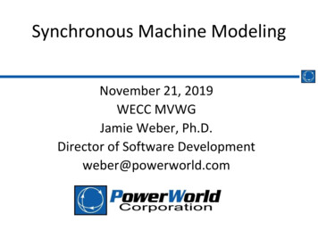
Magnetic Saturation andHysteresis The below image shows the saturationcurves for various materialsMagnetization curves of 9ferromagnetic materials, showingsaturation. 1.Sheet steel, 2.Siliconsteel, 3.Cast steel, 4.Tungsten steel,5.Magnet steel, 6.Cast iron,7.Nickel, 8.Cobalt, 9.Magnetite;highest saturation materials canget to around 2.2 or 2.3TImage Source:en.wikipedia.org/wiki/Saturation (magnetic)H is proportional to current60
Magnetic Saturation andHysteresis Magnetic materials also exhibit hysteresis, so thereis some residual magnetism when the current goesto zero; design goal is to reduce the area enclosedby the hysteresis loopTo minimize the amountof magnetic material,and hence cost andweight, electric machinesare designed to operateclose to saturationImage source: /MagParticle/Graphics/BHCurve.gif61
Typical Saturation Tests PlotTerminal Voltage vs. Efd For those doing generator testing they will do teststo build the figure on left, but I like to flip axes andthink about the figure on the right insteadVtermIfdIf at synchronous speed, thenTerminal Voltage has samemagnitude as stator fluxIfdVterm62
What is showing the Saturation? Saturation representshow extra field current isnecessary to obtain aparticular terminalvoltageIfd– It doesn’t follow the redline which would representa linear magneticrelationship The Saturation Functionwill be a function of Flux(Voltage) and representsthe green segmentsVterm63
Saturation is the “Extra” abovewhat linear term represents Saturation Function isdetermined fromgenerator testing bygetting the purple line atthe right Any function thatapproximates the purpleshape can be used Different software toolsand particular models usedifferent functionsEfdVterm64
Description of Saturation inSoftware Two points on the saturation curve areprovided as input data The saturation function is given. Can bedifferent types– Quadratic– Scaled Quadratic– ExponentialS12S101.01.265
Saturation Function TypesNameQuadraticFunction𝑆𝑎𝑡 𝑥 𝐵 𝑥 𝐴ScaledQuadratic𝐵 𝑥 𝐴𝑆𝑎𝑡 𝑥 𝑥Exponential𝑆𝑎𝑡 𝑥 𝐵𝑥 𝐴22Which PlatformGE PSLFPowerWorld SimulatoroptionPTI PSS/E,PowerWorld SimulatorOptionBPA IPFSpecific models in PTIPSS/ESpecific models inPowerWorld Simulator66
Scaled Quadratic Function 𝑆𝑎𝑡 𝑥 𝐵 𝑥 𝐴 2ቐ 𝑥0𝐼𝑓 𝑥 𝐴𝐼𝑓 𝑥 𝐴– A and B coefficients are calculated from the two equationsdefined by the two given points– There are two solutions though: we take the onerepresenting the Green Curve (A 1)𝐵 1.2 𝐴 2𝐵 1.0 𝐴 2𝑆12 𝑆10 1.21.0Solve one for B and substitute into the second. Groupsterms and you get quadratic function with twosolutions. Use the solution for which A 1.𝑆12𝑆12𝑆12 1.0 2 1.2 2 2 𝐴 𝐴 0𝑆10𝑆10𝑆10 1.267
Quadratic Function𝐵 𝑥 𝐴 𝑆𝑎𝑡 𝑥 ቊ02𝐼𝑓 𝑥 𝐴𝐼𝑓 𝑥 𝐴– A and B coefficients are calculated from the two equationsdefined by the two given points– There are two solutions though: we take the onerepresenting the Green Curve (A 1)𝑆10 𝐵 1.0 𝐴2𝑆12 𝐵 1.2 𝐴2Solve one for B and substitute into the second. Groupsterms and you get quadratic function with twosolutions. Use the solution for which A 1.𝑆12𝑆12𝑆12 1.44 2 2.4 𝐴 1.0 𝐴2 0𝑆10𝑆10𝑆1068
Exponential Function 𝑆𝑎𝑡 𝑥 𝐵 𝑥𝐴– A and B coefficients are calculated from the twoequations defined by the two given points𝑆10 𝐵 1.0𝐴B 𝑆10𝑆10 𝐵𝑆12 𝐵 1.2𝐴𝑆12 S10 1.2𝑆12 1.2𝑆10ln𝐴𝐴𝑆12 ln 1.2𝑆10𝐴 𝐴 ln 1.2𝑆12ln𝑆10𝐴 ln 1.269
Implementing Saturation Models When implementing saturation models incode, it is important to recognize that thefunction is meant to be positive, sonegative values are not allowed In large cases one is almost guaranteed tohave special cases, sometimes caused byuser typos– What to do if Se(1.2) Se(1.0)?– What to do if Se(1.0) 0 and Se(1.2) 0– What to do if Se(1.0) Se(1.2) 070
Where in Equations do you putSaturation: GENROU ExampleGENROU withSaturation71
Where in Equations do you putSaturation: GENROU Example72
Saturation is being Added to theSub-transient derivative Saturation is Added to theField Current– This makes senseespecially bec
–Book is too detailed for a classroom textbook, but it is a really great as a reference book once you’re working Another good theoretical book is Power System Dynamics and Stability by Peter Sauer and M.A. Pai from 1998. –The derivation in this book of the synchronous