Transcription
Basic Principles of Statistical InferenceKosuke ImaiDepartment of PoliticsPrinceton UniversityPOL572 Quantitative Analysis IISpring 2016Kosuke Imai (Princeton)Basic PrinciplesPOL572Spring 20161 / 66
What is Statistics?Relatively new disciplineScientific revolution in the 20th centuryData and computing revolutions in the 21st centuryThe world is stochastic rather than deterministicProbability theory used to model stochastic eventsStatistical inference: Learning about what we do not observe(parameters) using what we observe (data)Without statistics: wild guessWith statistics: principled guess123assumptionsformal propertiesmeasure of uncertaintyKosuke Imai (Princeton)Basic PrinciplesPOL572Spring 20162 / 66
Three Modes of Statistical Inference1Descriptive Inference: summarizing and exploring dataInferring “ideal points” from rollcall votesInferring “topics” from texts and speechesInferring “social networks” from surveys2Predictive Inference: forecasting out-of-sample data pointsInferring future state failures from past failuresInferring population average turnout from a sample of votersInferring individual level behavior from aggregate data3Causal Inference: predicting counterfactualsInferring the effects of ethnic minority rule on civil war onsetInferring why incumbency status affects election outcomesInferring whether the lack of war among democracies can beattributed to regime typesKosuke Imai (Princeton)Basic PrinciplesPOL572Spring 20163 / 66
Statistics for Social ScientistsQuantitative social science research:12345Find a substantive questionConstruct theory and hypothesisDesign an empirical study and collect dataUse statistics to analyze data and test hypothesisReport the resultsNo study in the social sciences is perfectUse best available methods and data, but be aware of limitationsMany wrong answers but no single right answerCredibility of data analysis:Data analysis assumption statistical theory interpretation {z} {z} {z}subjectiveobjectivesubjectiveStatistical methods are no substitute for good research designKosuke Imai (Princeton)Basic PrinciplesPOL572Spring 20164 / 66
Sample SurveysKosuke Imai (Princeton)Basic PrinciplesPOL572Spring 20165 / 66
Sample SurveysA large population of size NFinite population: N Super population: N A simple random sample of size nProbability sampling: e.g., stratified, cluster, systematic samplingNon-probability sampling: e.g., quota, volunteer, snowball samplingThe population: Xi for i 1, . . . , NSampling (binary) indicator: Z1 , . . . , ZNPAssumption: Ni 1 Zi n and Pr(Zi 1) n/N for all i N!# of combinations: Nn n!(N n)!Estimand population mean vs. Estimator sample mean:N1XX XiNi 1Kosuke Imai (Princeton)N1Xand x̄ Zi XinBasic Principlesi 1POL572Spring 20166 / 66
Estimation of Population MeanDesign-based inferenceKey idea: Randomness comes from sampling aloneUnbiasedness (over repeated sampling): E(x̄) XVariance of sampling distribution: S2n V(x̄) 1 n {z N }finite population correctionwhere S 2 PNi 1 (Xi X )2 /(N 1) is the population varianceUnbiased estimator of the variance: n s2σ̂ 2 1 and E(σ̂ 2 ) V(x̄)N nP2where s2 Ni 1 Zi (Xi x̄) /(n 1) is the sample variancePlug-in (sample analogue) principleKosuke Imai (Princeton)Basic PrinciplesPOL572Spring 20167 / 66
Some VERY Important Identities in Statistics1V(X ) E(X 2 ) {E(X )}22Cov(X , Y ) E(XY ) E(X )E(Y )3Law of Iterated Expectation:E(X ) E{E(X Y )}4Law of Total Variance:V(X ) E{V(X Y )} {z} within group variance5V{E(X Y )} {z}between group varianceMean Squared Error Decomposition:E{(θ̂ θ)2 } {E(θ̂ θ)}2 V(θ̂) {z} {z}bias2Kosuke Imai (Princeton)Basic PrinciplesvariancePOL572Spring 20168 / 66
Analytical Details of Randomization Inference123E(Zi ) E(Zi2 ) n/N and V(Zi ) E(Zi2 ) E(Zi )2 nN1 nN n(n 1)E(Zi Zj ) E(Zi Zj 1) Pr(Zj 1) N(N 1)for i 6 j and thus nCov(Zi , Zj ) E(Zi Zj ) E(Zi )E(Zj ) N(N 1) 1 NnUse these results to derive the expression:V(x̄) !NX1VZi Xin2i 1 NN XN XX12XV(Z) XXCov(Z,Z)iijiji n2 i 1i 1 j6 i !2 NN X X1 n 1NXi2 Xi1 nN N(N 1) i 1i 1 {z} S 2where we used the equalityKosuke Imai (Princeton)PNi 1 (XiBasic Principles X )2 PN2i 1 XiPOL572 NXSpring 201629 / 66
4Finally, we proceed as follows:E( NX)Zi (Xi x̄)2i 1 2 N X E Zi (Xi X ) (X x̄) {z} i 1 E( NXadd & subtract)Zi (Xi X )2 n(X x̄)2i 1 E( NX)2Zi (Xi X ) nV(x̄)i 1n(N 1) 2 n 2S 1 SNN (n 1)S 2 Thus, E(s2 ) S 2 , implying that the sample variance is unbiasedfor the population varianceKosuke Imai (Princeton)Basic PrinciplesPOL572Spring 201610 / 66
Inverse Probability WeightingUnequal sampling probability: Pr(Zi 1) πi for each iWe stillPrandomly sample n unitsPN from the population of size Nwhere NZ nimplyingi 1 ii 1 πi nOversampling of minorities, difficult-to-reach individuals, etc.Sampling weights inverse of sampling probabilityHorvitz-Thompson estimator:N1 X Zi Xix̃ Nπii 1Unbiasedness: E(x̃) XDesign-based variance is complicated but availableHáyek estimator (biased but possibly more efficient):PNZi Xi /πi x̃ Pi 1Ni 1 Zi /πiUnknow sampling probabilityKosuke Imai (Princeton)post-stratificationBasic PrinciplesPOL572Spring 201611 / 66
Model-Based InferenceAn infinite population characterized by a probability modelNonparametric FParametric Fθ (e.g., N (µ, σ 2 ))A simple random sample of size n: X1 , . . . , XnAssumption: Xi is independently and identically distributed (i.i.d.)according to FEstimator sample mean vs. Estimand population mean:n1Xµ̂ Xinandµ E(Xi )i 1Unbiasedness: E(µ̂) µVariance and its unbiased estimator:V(µ̂) σ2nnandσ̂ 2 i 1where σ 2 V(Xi )Kosuke Imai (Princeton)1 X(Xi µ̂)2n 1Basic PrinciplesPOL572Spring 201612 / 66
(Weak) Law of Large Numbers (LLN)If {Xi }ni 1 is a sequence of i.i.d. random variables with mean µ andfinite variance σ 2 , thenpX n µpwhere “ ” denotes the convergence in probability, i.e., ifpXn x, thenlim Pr( Xn x ) 0 for any 0n pIf Xn x, then for any continuous function f (·), we havepf (Xn ) f (x)Implication: Justifies the plug-in (sample analogue) principleKosuke Imai (Princeton)Basic PrinciplesPOL572Spring 201613 / 66
LLN in ActionIn Journal of Theoretical Biology,1234“Big and Tall Parents have More Sons” (2005)“Engineers Have More Sons, Nurses Have More Daughters” (2005)“Violent Men Have More Sons” (2006)“Beautiful Parents Have More Daughters” (2007)findings received broad attention inthe news media. For example, thepopular Freakonomics blog reported,Law of Averages in actionboys32 girls 2445 girls 35 boys24 girls 35bo19951996199721 girls 25 boys199823 girls 30 boys19991995:1996:1997:1998:1999:2000:ys29 girls 25 boys2000A new study by Satoshi Kanazawa, an evolutionary psychologistat the LondonSchool of Econom1ics, suggests . . . there are morebeautiful2 women in the worldthan there are handsome men.Why? Kanazawa argues it’s be3cause good-lookingparents are36 percent more likely to have a4baby daughter as their first childthan a baby son—which suggests,5evolutionarilyspeaking, thatbeauty is a trait more valuable forwomen6than for men. The studywas conducted with data from3,000 Americans, derived fromthe National Longitudinal Studyof Adolescent Health, and waspublished in the Journal of Theoretical Biology.57.1%56.651.850.649.350.0No dupilicates: 47.7%Population frequency: 48.5%Publication in a peer-reviewed jour-Figure 4. The authors performed a sex-ratio study of the offspring of the most beautiful peoplenal seemed to have removed all skeptiin the world as selected by People magazine between 1995 and 2000. The girls started strong incism, which is noteworthy given that1995 with 32 girls to 24 boys. Girls continued strong in 1996. However, as the sample size grew,the authors of Freakonomics are themthe ratio converged on the population frequency, concluding with 157 girls and 172 boys, orselves well qualified to judge social47.7 equencyof48.5percent.Kosuke Imai (Princeton)Basic PrinciplesPOL572Gelman & Weakliem, American Scientistscience research.Spring 201614 / 66
Central Limit Theorem (CLT)If {Xi }ni 1 is a sequence of i.i.d. random variables with mean µ andfinite variance σ 2 , thenXn µ σ/ n {z }d N (0, 1)z-score of sample meandwhere “ ” represents the convergence in distribution, i.e., ifdXn X , thenlim P(Xn x) P(X x) for all xn with P(X x) being continuous at every xdIf Xn X , then for any continuous function f (·),df (Xn ) f (X )Implication: Justifies asymptotic (normal) approximationKosuke Imai (Princeton)Basic PrinciplesPOL572Spring 201615 / 66
CLT in Actionnth row and k th column n 1k 1 # of ways to get there Binomial distribution: Pr(X k ) kn pk (1 p)n kSir Francis Galton’s Quincunx, Boston Museum of Science, or justcheck out YouTubeKosuke Imai (Princeton)Basic PrinciplesPOL572Spring 201616 / 66
Asymptotic Properties of the Sample Meani.i.d.The Model: Xi Fµ,σ2LLN implies consistency:pµ̂ X n µCLT implies asymptotic normality: dn(µ̂ µ) N (0, σ 2 ) σ2approx. µ̂ N µ,nin a large sampleBut, σ is unknownStandard error: estimated standard deviation of samplingdistributionσ̂s.e. nwhere σ̂ 2 is unbiased (shown before) and consistent for σ 2 (LLN)Kosuke Imai (Princeton)Basic PrinciplesPOL572Spring 201617 / 66
Asymptotic Confidence IntervalsPutting together, we have:µ̂ µ d N (0, 1)σ̂/ n {z }z scorepdWe used the Slutzky Theorem: If Xn x and Yn Y , thenddXn Yn x Y and Xn Yn xYThis gives 95% asymptotic confidence interval: µ̂ µpPr 1.96 1.96 0.95σ̂/ n p Pr µ̂ 1.96 σ̂/ n µ µ̂ 1.96 σ̂/ n 0.95Kosuke Imai (Princeton)Basic PrinciplesPOL572Spring 201618 / 66
(1 α) 100% asymptotic confidence interval (symmetric andbalanced):CI1 α [µ̂ zα/2 s.e.,µ̂ zα/2 s.e.]where s.e. represents the standard errorCritical value: Pr(Z zα/2 ) Φ( zα/2 ) α/2 where Z N (0, 1)123α 0.01 gives zα/2 2.58α 0.05 gives zα/2 1.96α 0.10 gives zα/2 1.64Be careful about the interpretation!Confidence intervals are random, while the truth is fixedProbability that the true value is in a particular confidence interval iseither 0 or 1 and not 1 αpNominal vs. actual coverage probability: Pr(µ CI1 α ) 1 αAsymptotic inference approximate inferenceKosuke Imai (Princeton)Basic PrinciplesPOL572Spring 201619 / 66
Exact Inference with Normally Distributed DataSometimes, exact model-based inference is possiblei.i.d.If Xi N (µ, σ 2 ), then µ̂ N (µ, σ 2 /n) in a finite sampleMoreover, in a finite sample,t statistic µ̂ µ σ̂/ nexactly tn 1where tn 1 is the t distribution with n 1 degrees of freedomUse tn 1 (rather than N (0, 1)) to obtain the critical value for exactconfidence intervalsAs n increases, tn 1 approaches to N (0, 1)Fat tail: more conservative inference with wider CISum of independent random variables: Bernoulli (Binomial),Exponential (Gamma), Poisson (Poisson), χ2 (χ2 ), etc.Kosuke Imai (Princeton)Basic PrinciplesPOL572Spring 201620 / 66
0.10.2n 2n 10n 500.0density0.30.4Student’s t Distribution 6Kosuke Imai (Princeton) 4 20Basic Principles2POL57246Spring 201621 / 66
Application: Presidential Election Polling2000 Butterfly ballot debacle: Oops, we have this system calledelectoral college!National polls state pollsForecasting fun: political methodologists, other “statisticians”Idea: estimate probability that each state is won by a candidateand then aggregate electoral votesQuantity of interest: Probability of a candidate winning the electionKosuke Imai (Princeton)Basic PrinciplesPOL572Spring 201622 / 66
Simple Model-Based InferenceSetup: njk respondents of poll j from state kModel for # of Obama supporters in poll j and state k :Xjkindep. Binom(njk , pk )Parameters of interest: θ {p1 , p2 , . . . , p51 }Popular methods of inference:123Method of moments (MM) solve the moment equationsample moments(X ) population moments(θ)Maximum likelihood (ML) maximize the likelihood f (X θ)Bayesian inference derive the posterior of parameterslikelihoodf (θ X ) marginal likelihood In this case, MM and ML give p̂k Kosuke Imai (Princeton)priorz } {z} {f (X θ) f (θ)f (X ) {z}RBasic Principles f (X θ) f (θ)f (X θ)f (θ)dθPJkj 1 Xjk /PJkj 1 njkPOL572Spring 201623 / 66
Estimated Probability of Obama Victory in 2008Estimate pk for each stateSimulate M elections using p̂k and its standard error:12\for state k , sample Obama’s voteshare from N (p̂k , V(p̂k ))collect all electoral votes from winning statesPlot M draws of total electoral votesActual # ofEVs won0.04mean 353.28sd 11.720.000.02Density0.060.08Distribution of Obama's Predicted Electoral Votes320340360380Electoral VotesKosuke Imai (Princeton)Basic PrinciplesPOL572Spring 201624 / 66
Nominal vs. Actual Coverage80Poll Results versus the Actual Election Results60 Bias: 1 ppt.020 20Poll Results40Coverage: 55% Bias-adjustedcoverage: 60% Still significantundercoverage 20020406080Actual Election ResultsKosuke Imai (Princeton)Basic PrinciplesPOL572Spring 201625 / 66
Key PointsRandom sampling enables statistical inferenceDesign-based vs. Model-based inference12Design-based: random sampling as basis for inferenceModel-based: probability model as basis for inferenceSampling weights: inverse probability weightingChallenges of survey research:cluster sampling, multi-stage sampling loss of efficiencystratified samplingunit non-responsenon-probability sampling model-based inferenceitem non-response, social desirability bias, etc.Kosuke Imai (Princeton)Basic PrinciplesPOL572Spring 201626 / 66
Causal InferenceKosuke Imai (Princeton)Basic PrinciplesPOL572Spring 201627 / 66
What is Causal Inference?Comparison between factual and counterfactual for each unitIncumbency effect:What would have been the election outcome if a candidate werenot an incumbent?Resource curse thesis:What would have been the GDP growth rate without oil?Democratic peace theory:Would the two countries have escalated crisis in the samesituation if they were both autocratic?S UPPLEMENTARY READING: Holland, P. (1986). Statistics andcausal inference. (with discussions) Journal of the AmericanStatistical Association, Vol. 81: 945–960.Kosuke Imai (Princeton)Basic PrinciplesPOL572Spring 201628 / 66
Defining Causal EffectsUnits: i 1, . . . , n“Treatment”: Ti 1 if treated, Ti 0 otherwiseObserved outcome: YiPre-treatment covariates: XiPotential outcomes: Yi (1) and Yi (0) where Yi Yi (Ti )Votersi123.ContactTi100.n1TurnoutYi (1) Yi (0)1?0?1.0?AgeXi205540.Party IDXiDRR.62DCausal effect: Yi (1) Yi (0)Kosuke Imai (Princeton)Basic PrinciplesPOL572Spring 201629 / 66
The Key AssumptionsThe notation implies three assumptions:123No simultaneity (different from endogeneity)No interference between units: Yi (T1 , T2 , . . . , Tn ) Yi (Ti )Same version of the treatmentStable Unit Treatment Value Assumption (SUTVA)Potential violations:123feedback effectsspill-over effects, carry-over effectsdifferent treatment administrationPotential outcome is thought to be “fixed”: data cannot distinguishfixed and random potential outcomesPotential outcomes across units have a distributionObserved outcome is random because the treatment is randomMulti-valued treatment: more potential outcomes for each unitKosuke Imai (Princeton)Basic PrinciplesPOL572Spring 201630 / 66
Causal Effects of Immutable Characteristics“No causation without manipulation” (Holland, 1986)Immutable characteristics; gender, race, age, etc.What does the causal effect of gender mean?Causal effect of having a female politician on policy outcomes(Chattopadhyay and Duflo, 2004 QJE)Causal effect of having a discussion leader with certainpreferences on deliberation outcomes (Humphreys et al. 2006WP)Causal effect of a job applicant’s gender/race on call-back rates(Bertrand and Mullainathan, 2004 AER)Problem: confoundingKosuke Imai (Princeton)Basic PrinciplesPOL572Spring 201631 / 66
Average Treatment EffectsSample Average Treatment Effect (SATE):n1X(Yi (1) Yi (0))ni 1Population Average Treatment Effect (PATE):E(Yi (1) Yi (0))Population Average Treatment Effect for the Treated (PATT):E(Yi (1) Yi (0) Ti 1)Treatment effect heterogeneity: Zero ATE doesn’t mean zeroeffect for everyone! Conditional ATEOther quantities: Quantile treatment effects etc.Kosuke Imai (Princeton)Basic PrinciplesPOL572Spring 201632 / 66
Design ConsiderationsRandomized experimentsLaboratory experimentsSurvey experimentsField experimentsObservational studiesTradeoff between internal and external validityEndogeneity: selection biasGeneralizability: sample selection, Hawthorne effects, realism“Designing” observational studiesNatural experiments (haphazard treatment assignment)Examples: birthdays, weather, close elections, arbitraryadministrative rulesGeneralizing experimental results: possible extrapolationBottom line: No study is perfect, statistics is always neededKosuke Imai (Princeton)Basic PrinciplesPOL572Spring 201633 / 66
(Classical) Randomized ExperimentsUnits: i 1, . . . , nMay constitute a simple random sample from a populationTreatment: Ti {0, 1}Outcome: Yi Yi (Ti )Complete randomization of the treatment assignmentExactly n1 units receive the treatmentn0 n n1 units are assigned to the control groupPAssumption: for all i 1, . . . , n, ni 1 Ti n1 and(Yi (1), Yi (0)) Ti ,Pr(Ti 1) n1nEstimand SATE or PATEEstimator Difference-in-means:nn1 X1 Xτ̂ Ti Yi (1 Ti )Yin1n0i 1Kosuke Imai (Princeton)Basic Principlesi 1POL572Spring 201634 / 66
Unbiased Estimation of Average Treatment EffectsKey idea (Neyman 1923): Randomness comes from treatmentassignment (plus sampling for PATE) aloneDesign-based (randomization-based) rather than model-basedStatistical properties of τ̂ based on design featuresDefine O {Yi (0), Yi (1)}ni 1Unbiasedness (over repeated treatment assignments):E(τ̂ O) nn1 X1 XE(Ti O)Yi (1) {1 E(Ti O)}Yi (0)n1n01ni 1nXi 1(Yi (1) Yi (0))i 1 SATEKosuke Imai (Princeton)Basic PrinciplesPOL572Spring 201635 / 66
Randomization Inference for SATEVariance of τ̂ :V(τ̂ O) 1n n0 2 n1 2S S 2S01 ,n1 1 n0 0where for t 0, 1,nSt2S01 1 X(Yi (t) Y (t))2n 11n 1i 1nXsample variance of Yi (t)(Yi (0) Y (0))(Yi (1) Y (1)) sample covariancei 1The variance is NOT identifiableKosuke Imai (Princeton)Basic PrinciplesPOL572Spring 201636 / 66
The usual variance estimator is conservative on average:S12 S02 n1n0V(τ̂ O) Under the constant additive unit causal effect assumption, i.e.,Yi (1) Yi (0) c for all i,S01 1 2(S S02 ) and2 1V(τ̂ O) S12 S02 n1n0The optimal treatment assignment rule:n1opt Kosuke Imai (Princeton)n,1 S0 /S1n0opt Basic Principlesn1 S1 /S0POL572Spring 201637 / 66
Details of Variance Derivation1Let Xi Yi (1) n1 Yi (0)/n0 and Di nTi /n1 1, and write !2n 1 XOV(τ̂ O) EDXi i n2 i 12ShowE(Di O) 0,E(Di Dj O) 3E(Di2 O) n0,n1n0n1 (n 1)Use Ê and Ë to show,V(τ̂ O) nXn0(Xi X )2n(n 1)n1i 14Substitute the potential outcome expressions for XiKosuke Imai (Princeton)Basic PrinciplesPOL572Spring 201638 / 66
Randomization Inference for PATENow assume that units are randomly sampled from a populationUnbiasedness (over repeated sampling):E{E(τ̂ O)} E(SATE) E(Yi (1) Yi (0)) PATEVariance:V(τ̂ ) V(E(τ̂ O)) E(V(τ̂ O))σ12 σ02 n1n0where σt2 is the population variance of Yi (t) for t 0, 1Kosuke Imai (Princeton)Basic PrinciplesPOL572Spring 201639 / 66
Asymptotic Inference for PATEHold k n1 /n constantRewrite the difference-in-means estimator as n 1 X Ti Yi (1) (1 Ti )Yi (0)τ̂ nk1 ki 1 {z}i.i.d. with mean PATE & variance nV(τ̂ )Consistency:pτ̂ PATEAsymptotic normality: dn(τ̂ PATE) Nσ02σ20, 1 k1 k!(1 α) 100% Confidence intervals:[τ̂ s.e. zα/2 , τ̂ s.e. zα/2 ]Kosuke Imai (Princeton)Basic PrinciplesPOL572Spring 201640 / 66
Model-based Inference about PATEA random sample of n1 units from the “treatment” population ofinfinite sizeA random sample of n0 units from the “control” population ofinfinite sizeThe randomization of the treatment implies that two populationsare identical except the receipt of the treatmentThe difference in the population means PATEUnbiased estimator from the model-based sample surveys:τ̂ n0n11 X1 XY0iY1i n1n0i 1i 1Variance is identical: V(τ̂ ) Kosuke Imai (Princeton)σ12n1 σ02n0Basic PrinciplesPOL572Spring 201641 / 66
Identification vs. EstimationObservational studies No randomization of treatmentDifference in means between two populations can still beestimated without biasValid inference for ATE requires additional assumptionsLaw of Decreasing Credibility (Manski): The credibility of inferencedecreases with the strength of the assumptions maintainedIdentification: How much can you learn about the estimand if youhad an infinite amount of data?Estimation: How much can you learn about the estimand from afinite sample?Identification precedes estimationKosuke Imai (Princeton)Basic PrinciplesPOL572Spring 201642 / 66
Identification of the Average Treatment EffectAssumption 1: Overlap (i.e., no extrapolation)0 Pr(Ti 1 Xi x) 1 for any x XAssumption 2: Ignorability (exogeneity, unconfoundedness, noomitted variable, selection on observables, etc.){Yi (1), Yi (0)} Ti Xi x for any x XUnder these assumptions, we have nonparametric identification:τ E{µ(1, Xi ) µ(0, Xi )}where µ(t, x) E(Yi Ti t, Xi x)Kosuke Imai (Princeton)Basic PrinciplesPOL572Spring 201643 / 66
Partial IdentificationPartial (sharp bounds) vs. Point identification (point estimates):123What can be learned without any assumption other than the oneswhich we know are satisfied by the research design?What is a minimum set of assumptions required for pointidentification?Can we characterize identification region if we relax some or all ofthese assumptions?ATE with binary outcome:[ Pr(Yi 0 Ti 1, Xi x)π(x) Pr(Yi 1 Ti 0, Xi x){1 π(x)},Pr(Yi 1 Ti 1, Xi x)π(x) Pr(Yi 0 Ti 0, Xi x){1 π(x)}]where π(x) Pr(Ti 1 Xi x) is called propensity scoreThe width of the bounds is 1: “A glass is half empty/full”Kosuke Imai (Princeton)Basic PrinciplesPOL572Spring 201644 / 66
Application: List ExperimentThe 1991 National Race and Politics Survey (Sniderman et al.)Randomize the sample into the treatment and control groupsThe script for the control groupNow I’m going to read you three things that sometimesmake people angry or upset. After I read all three,just tell me HOW MANY of them upset you. (I don’twant to know which ones, just how many.)(1) the federal government increasing the tax ongasoline;(2) professional athletes getting million-dollar-plussalaries;(3) large corporations polluting the environment.Kosuke Imai (Princeton)Basic PrinciplesPOL572Spring 201645 / 66
Application: List ExperimentThe 1991 National Race and Politics Survey (Sniderman et al.)Randomize the sample into the treatment and control groupsThe script for the treatment groupNow I’m going to read you four things that sometimesmake people angry or upset. After I read all four,just tell me HOW MANY of them upset you. (I don’twant to know which ones, just how many.)(1) the federal government increasing the tax ongasoline;(2) professional athletes getting million-dollar-plussalaries;(3) large corporations polluting the environment;(4) a black family moving next door to you.Kosuke Imai (Princeton)Basic PrinciplesPOL572Spring 201646 / 66
Identification Assumptions and Potential OutcomesIdentification assumptions:1No Design Effect: The inclusion of the sensitive item does not affectanswers to control items2No Liars: Answers about the sensitive item are truthfulDefine a type of each respondent bytotal number of yes for control items Yi (0)truthful answer to the sensitive item Zi Under the above assumptions, Yi (1) Yi (0) Zi A total of (2 (J 1)) typesKosuke Imai (Princeton)Basic PrinciplesPOL572Spring 201647 / 66
Example with 3 Control ItemsJoint distribution of πyz (Yi (0) y , Zi z) is identified:Yi43210Treatment group(3,1)(2,1) (3,0)(1,1) (2,0) (1,0) (0,1) (0,0) Control group(3,1)(2,1)(1,1) (0,1) (3,0)(2,0) (1,0) (0,0) Testing the validity of the identification assumptions: if theassumptions are valid, πyz should be positive for all y and zSuppose that a negative value of π̂yz is observed. Did this happenby chance?Statistical hypothesis test (next topic)Kosuke Imai (Princeton)Basic PrinciplesPOL572Spring 201648 / 66
Key PointsCausal inference is all about predicting counter-factualsAssociation (comparison between treated and control groups) isnot causation (comparison between factuals and counterfactuals)Randomization of treatment eliminates both observed andunobserved confoundersDesign-based vs. model-based inferenceObservational studies identification problemImportance of research design: What is your identificationstrategy?Kosuke Imai (Princeton)Basic PrinciplesPOL572Spring 201649 / 66
Statistical Hypothesis TestKosuke Imai (Princeton)Basic PrinciplesPOL572Spring 201650 / 66
Paul the Octopus and Statistical Hypothesis Tests2010 World CupGroup: Germany vs AustraliaGroup: Germany vs SerbiaGroup: Ghana vs GermanyRound of 16: Germany vs EnglandQuarter-final: Argentina vs GermanySemi-final: Germany vs Spain3rd place: Uruguay vs GermanyFinal: Netherlands vs SpainQuestion: Did Paul the Octopus get lucky?Suppose that Paul is randomly choosing winnerThen, # of correct answers Binomial(8, 0.5)The probability that Paul gets them all correct:Tie is possible in group rounds:133 125128 0.004 0.001Conclusion: Paul may be a prophetKosuke Imai (Princeton)Basic PrinciplesPOL572Spring 201651 / 66
What are Statistical Hypothesis Tests?Probabilistic “Proof by contradiction”General procedure:1Choose a null hypothesis (H0 ) and an alternative hypothesis (H1 )2Choose a test statistic Z3Derive the sampling distribution (or reference distribution) of Zunder H0Is the observed value of Z likely to occur under H0 ?4Yes Retain H0 (6 accept H0 )No Reject H0Kosuke Imai (Princeton)Basic PrinciplesPOL572Spring 201652 / 66
More Data about PaulReference distribution: Binom(14, 0.5)0.150.100.050.00A total of 14 matchesDensityGroup: Germany vs PolandGroup: Croatia vs GermanyGroup: Austria vs GermanyQuarter-final: Portugal vs GermanySemi-final: Germany vs TurkeyFinal: Germany vs Spain0.20UEFA Euro 200812 correct guesses02468101214Number of correct guessesp-value: Probability that under the null you observe something atleast as extreme as what you actually observedPr({12, 13, 14}) 0.001In R: pbinom(12, size 14, prob 0.5, lower.tail FALSE)Kosuke Imai (Princeton)Basic PrinciplesPOL572Spring 201653 / 66
p-value and Statistical Significancep-value: the probability, computed under H0 , of observing a valueof the test statistic at least as extreme as its observed valueA smaller p-value presents stronger evidence against H0p-value less than α indicates statistical significance at thesignificance level αp-value is NOT the probability that H0 (H1 ) is true (false)A large p-value can occur either because H0 is true or because H0is false but the test is not powerfulThe statistical significance indicated by the p-value does notnecessarily imply scientific significanceInverting the hypothesis test to obtain confidence intervalsTypically better to present confidence intervals than p-valuesKosuke Imai (Princeton)Basic PrinciplesPOL572Spring 201654 / 66
One-Sample TestLooks and politics: Todorov et al. Sciencep probability that a more competent politician winsH0 : p 0.5 and H1 : p 0.5Test statistic p̂ sample proportionExact reference distribution: p̂ Binom(n, 0.5)Asymptotic reference distribution via CLT:Z statistic Kosuke Imai (Princeton)p̂ 0.5p̂ 0.5 d N (0, 1) s.e.0.5/ nBasic PrinciplesPOL572Spring 201655 / 66
Two-Sample TestH0 : PATE τ0 and H1 : PATE 6 τ0Difference-in-means estimator: τ̂Asymptotic reference distribution:Z statistic τ̂ τ0τ̂ τ0d r N (0, 1)s.e.22σ̂0σ̂1n1 n0Is Zobs unusual under the null?Reject the null when Zobs z1 α/2Retain the null when Zobs z1 α/2i.i.d.i.i.d.If we assume Yi (1) N (µ1 , σ12 ) and Yi (0) N (µ0 , σ02 ), thent statistic τ̂ τ0 tνs.e.where ν is given by a complex formula (Behrens-Fisher problem)Kosuke Imai (Princeton)Basic PrinciplesPOL572Spring 201656 / 66
Lady Tasting TeaDoes tea taste different depending on whether the tea was pouredinto the milk or whether the milk was poured into the tea?8 cups; n 8Randomly choose 4 cups into which pour the tea first (Ti 1)Null hypothesis: the lady cannot tell the differenceSharp null – H0 : Yi (1) Yi (0) for all i 1, . . . , 8Statistic: the number of correctly classified cupsThe lady classified all 8 cups correctly!Did this happen by chance?Example: Ho and Imai (2006). “Randomization Inference withNatural Experiments: An Analysis of Ballot Effects in the 2003California Recall Election.” J. of the Amer. Stat. Assoc.Kosuke Imai (Princeton)Basic PrinciplesPOL572Spring 201657 / 66
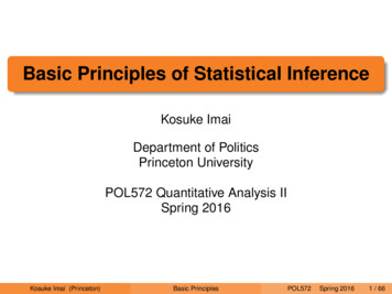
Randomization Test (Fisher’s Exact Test)8 C4Probability Distribution0.40.3probability0.20.10.0205 100frequency30actual scenarios . . .MTTTTTTTTMTMMMMTMMTMT02468MMM8 Number4of correctly6guessed cups0.5Frequency Plotcupsguess1M2T3T4M5M6T7T8Mcorrectly guessed02468Number of correctly guessed cups 70 ways to do this and each arrangement is equally likelyWhat is the p-value?No assumption, but the sharp null may be of little interestKosuke Imai (Princeton)Basic PrinciplesPOL572Spring 201658 / 66
Error and Power of Hypothesis TestTwo types of errors:H0 is trueH0 is falseReject H0Type I e
Statistics for Social Scientists Quantitative social science research: 1 Find a substantive question 2 Construct theory and hypothesis 3 Design an empirical study and collect data 4 Use statistics to analyze data and test hypothesis 5 Report the results No study in the social sciences is perfect Use bes