Transcription
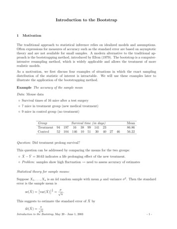
Introduction to the Bootstrap1MotivationThe traditional approach to statistical inference relies on idealized models and assumptions.Often expressions for measures of accuracy such as the standard error are based on asymptotictheory and are not available for small samples. A modern alternative to the traditional approach is the bootstrapping method, introduced by Efron (1979). The bootstrap is a computerintensive resampling method, which is widely applicable and allows the treatment of morerealistic models.As a motivation, we first discuss four examples of situations in which the exact samplingdistribution of the statistic of interest is intractable. We will use these examples later toillustrate the application of the bootstrapping method.Example The accuracy of the sample meanData: Mouse data Survival times of 16 mice after a test surgery 7 mice in treatment group (new medical treatment) 9 mice in control group (no treatment)GroupSurvival time (in days)Treatment 94 197 16 38 99 141 23Control52 104 146 10 51 30 402746Mean86.8656.22Question: Did treatment prolong survival?This question can be addressed by comparing the means for the two groups: X̄ Ȳ 30.63 indicates a life prolonging effect of the new treatment. Problem: samples show high fluctuationneed to assess accuracy of estimatesStatistical theory for sample means:Suppose X1 , . . . , Xn is an iid random sample with mean µ and variance σ 2 . Then the standarderror is the sample mean is 1σse(X̄) var(X̄) 2 .nThis suggests to estimate the standard error of X̄ bysnse(b X̄) Introduction to the Bootstrap, May 20 - June 1, 2003-1-
Pn12where s2 n 1i 1 (Xi X̄) . The interpretation of the standard error as a measure ofstatistical accuracy is based on the central limit theorem, which (under quite general conditionson the distribution of the Xi ) states that for large sample sizes n the sample mean X̄ isapproximately normally distributed, X̄ N µ, σ/ n .Thus we expect the mean X̄ to be within two standard errors of the mean µ about 95% of thetime. Substituting the above estimate for the standard error, we obtain a (1 α) confidenceinterval for µ,b X̄).X̄ tn 1, α2 se(In the mouse data example, we are interested in the question whether the new treatment leadto an increase in survival time. For this, we might consider the studentized test statisticT pX̄ Ȳse(b X̄)2 se(b Ȳ )2.The observed value of T is 1.05, which indicates that the effect of the new treatment on survivalis not significant.Problems: The exact distribution of the two-sample test statistic T is not known (there are a numberof approximations like Satterthwaite’s approximation).Example Accuracy of the sample medianSuppose that we want to compare the treatment and the control group in the mouse dataexample by their medians rather than their means. From the table above we findmed(X) 94,med(Y ) 46,andT 0 med(X) med(Y ) 48.In order to decide whether this is a significant difference, we need to quantify the accuracy ofthe sample medians.Statistical theory for sample medians Unlike in the case of the sample mean there is no small sample formula for the standarderror of the sample median. Suppose that the distribution P of the Xi is continuous with density p(x). Then for largen, the median is approximately normally distributed, med(X) N mP ,σ2,4n p(mP )2 where mP is the median of the distribution P (i.e. P(Xi mP ) 12and P(Xi mP ) 12 ).Problems:Introduction to the Bootstrap, May 20 - June 1, 2003-2-
Are 7 (or 9) observations enough for the asymptotic approximation to work well? Can we reliably estimate the density p at mp ? How does the estimation of the (asymptotic) standard error affect the width of the confidenceinterval based on the normal approximation?Example Maximum likelihood estimation using the EM algorithmConsider a missing data problem with observed data Yobs and missing data Ymis . If observationsare missing at random, the maximum likelihood estimator is derived from the observed-datalog-likelihood functionZln (θ Yobs ) p(Yobs , ymis θ) dymis ,where p(yobs , ymis θ) is the density of the complete data Y (Yobs , Ymis )T . For large samples,the maximum likelihood estimator θ̂ is approximately normally distributed,θ̂ θ0 N (0, Iobs (θ0 ) 1 )where θ0 is the true parameter (assuming the model is correct) and 2 ln (θ Yobs )Iobs (θ0 ) E θ2θ θ0is the observed information.Problems: For many missing-data problems, the observed-data log-likelihood is too difficult to evaluate,and inference is based on the iterative EM algorithm instead. The EM algorithm does not automatically provide standard errors associated with theparameter estimates. The asymptotic covariance matrix Iobs (θ0 ) 1 is not readily availablebecause the implementation of the EM algorithm is based on the complete-data problemand does not require the evaluation of the observed-data log-likelihood or its derivatives. The EM algorithm can be extended to estimate also the observed information (eg SEMalgorithm). This can be cumbersome.Example Number of modes of a densitySuppose that X1 , . . . , Xn are an iid sample from a distribution P with continuous density p(x).One important parameter of P is the number of modes of its density p(x). Multimodality ofthe density indicates a heterogeneity in the data. As an illustration, we consider the followingexample.Data: Galaxy data Velocities in km/sec of 82 galaxies from 6 well-separated conic sections of an unfilled surveyof the Corona Borealis region. Multimodality in the distribution of velocities is evidence for voids and superclusters in thefar universe.Introduction to the Bootstrap, May 20 - June 1, 2003-3-
In this example, the structure in the distribution of velocities corresponds to the spatial distribution of galaxies in the far universe. Thus the question of existence of voids and superclusterscan be addressed by testingH0 : nmode (p) 1vsHa : nmode (p) 1where nmode (p) is the number of modes of the density.The density of the velocities can be estimated nonparametrically by a kernel estimaten1 Px Xip̂K,h (x) K.nh i 1h The bandwidth h determines the resolution of the density estimate. The following figure showskernel estimates of the galaxy data for three different bandwidths.Kernel estimate (h 3.05)0.20Kernel estimate (h 1.0)Kernel estimate (h 0.6)Density0.150.100.050.00010203040Velocity of galaxy (1000km/s)As can be seen from the graphs, the number of modes exhibited by the density estimate p̂K,hdepends on the bandwidth h: For small h the estimate shows many modes some of which maybe attributed to chance variation in the data, whereas for large h the estimate is much smootherbut may exhibit too few modes due to oversmoothing. In particular, we can choose h largeenough such that p̂K,h only has one mode.Let H1 be the minimal bandwidth which leads to a unimodal density estimate, that is,nmode (p̂K,H1 ) 1andnmode (p̂K,h ) 1 for all h H1 .Note that H1 depends on X and is thus a random variable. Furthermore, let h1 be the observedvalue for H1 . Large values of h1 indicate oversmoothing and thus multimodality of the truedensity p. Thus H1 can be used as a test statistic for the above test problem and the nullhypothesis of unimodality is rejected at significance level α ifP(H1 h1 H0) α.Problem: Distribution of H1 under the null hypothesis H0 is unknown.2The Bootstrap PrincipleThe basic idea of the bootstrapping method is that, in absence of any other information aboutthe distribution, the observed sample contains all the available information about the underlyingIntroduction to the Bootstrap, May 20 - June 1, 2003-4-
distribution, and hence resampling the sample is the best guide to what can be expected fromresampling from the distribution.Suppose that a sample X (X1 , . . . , Xn )T is used to estimate a parameter θ of the distributionand let θ̂ s(X) be a statistic that estimates θ. For the purpose of statistical inference onθ, we are interested in the sampling distribution of θ̂ (or certain aspects of it) so as to assessthe accuracy of our estimator or to set confidence intervals for our estimate of θ. In manyapplications, however, the sampling distribution of θ̂ is intractable.If the true distribution P were known, we could draw samples X (b) ,use Monte Carlo methods to estimate the sampling distribution ofis unknown and we cannot sample from it, the bootstrapping ideaoriginal sample instead. This distribution from which the bootstrapempirical distribution.b 1, . . . , B from P andour estimate θ̂. Since Psuggests to resample thesamples are drawn is theThe empirical distribution For an sample X1 , . . . , Xn of independent real-valued randomvariables with distribution P , we define a probability distribution P̂ byP̂ (A) n1P1A (Xi ),n i 1for (appropriate) A R.P̂ is called the empirical distribution of the sample X. P̂ can be thought as the distributionwhich puts mass 1/n on each observation Xi (for values that occurs more than once in the samplethe mass will be a multiple of 1/n). It follows that P̂ is a discrete probability distribution witheffective sample space {X1 , . . . , Xn }.It can be shown that P̂ is a nonparametric maximum likelihood estimator of P which justifiesto estimate P by P̂ if no other information about P is available (such as e.g. P belongs to aparametric family).Theoretical results: Let A R (such that P (A) is defined, i.e. A belongs to the Borel σ-algebra).Then we haveP̂ (A) P (A)as n .This result is a direct consequence of the law of large numbers sincen P̂ (A) nP1A (Xi ) Bin(n, P (A))i 1and thus P̂ (A) tends to its expectation P (A) as n . This results can be strengthened tosup P̂ (A) P (A) 0as n ,A Iwhere I is the set of all intervals of R. In other words, the distribution P (A) can be approximated by P̂ (A) equally well for all A I.Sampling from the empirical distribution P̂ : Suppose we want to draw an iid sample X (X1 , . . . , Xn )T from P̂ . As we have noted above, P̂ puts mass 1/n on each observation Xi .Thus when sampling from P̂ , the ith observation Xi in the original sample is selected withprobability 1/n. This leads to the following two-step procedure:Introduction to the Bootstrap, May 20 - June 1, 2003-5-
Draw i1 , . . . , in independently from the uniform distribution on {1, . . . , n}. Set Xj Xij and X (X1 , . . . , Xn )T .In other words, we sample with replacement from the original sample X1 , . . . , Xn .The bootstrap principle Suppose that X (X1 , . . . , Xn )T is a random sample from a distribution P , θ t(P ) is some parameter of the distribution, θ̂ s(X) is an estimator for θ.For an evaluation of the statistical properties (such as bias or standard error) of the actualestimate θ̂, we wish to estimate the sampling distribution of θ̂.The bootstrapping method mimics the data-generating process by sampling from an estimateP̂ of the unknown distribution P . Thus the role of the above real quantities is taken by theiranalogous quantities in the “bootstrap world”: X (X1 , . . . , Xn )T is a bootstrap sample from P̂ , θ t(P̂ ) is the parameter in the bootstrap world, θ̂ s(X ) is the bootstrap replication of θ.The sampling distribution of θ̂ is then estimated by its bootstrap equivalentP̂(θ̂ A) P (θ̂ A).The bootstrap principle can be summarized by the following schematic diagram:Bootstrap WorldReal WorldUnknownprobabilitydistributionObserved randomsampleP X (X1 , . . . , Xn )BootstrapsampleEmpiricaldistribution P̂ X (X1 , . . . , Xn ) θ̂ s(X)θ̂ s(X )Statistic of interestBootstrap replicationIn general, the estimate P̂ will be determined by the available information about P . Only if thedata comprise all available information about P , we estimate P by the empirical distribution.Monte Carlo Approximation: Even though the distribution of the bootstrap sample X isknown, the evaluation of the exact bootstrap sampling distribution of θ̂ can be still intractable.In fact, the sampling distribution has been derived only for special cases such as the median ofan uneven number of observations.In general, the bootstrap estimate of the sampling distribution of θ̂ is computed using MonteCarlo methods:Introduction to the Bootstrap, May 20 - June 1, 2003-6-
Draw B independent bootstrap samples X (1) , . . . , X (B) from P̂ : (b)X1iid, . . . , Xn (b) P̂b 1, . . . , B Evaluate bootstrap replicationsθ̂ (b) s(X (b) )b 1, . . . , B Estimate the sampling distribution of θ̂ by the empirical distribution of the bootstrap replications θ̂ (1) , . . . , θ̂ (B) :P̂(θ̂ A) B1 P 1AB θ̂ (b) .b 1for appropriate subsets A Rp (if θ̂ Rp ).Often we are only interested in one characteristic of the sampling distribution of θ̂, for examplethe standard error or the bias. Estimates for these quantities can be straightforwardly obtainedfrom the bootstrap replications.The bootstrap algorithm for estimating standard errors Let θ̂ s(X) be an estimatorfor θ and suppose we want to know the standard error of θ̂. A bootstrap estimate of standarderror can be obtained by the following algorithm: Draw B independent bootstrap samples X (1) , . . . , X (B) from P̂ : (b)X1iid, . . . , Xn (b) P̂b 1, . . . , B. Evaluate the bootstrap replicationsθ̂ (b) s(X (b) )b 1, . . . , B. Estimate the standard error se(θ̂) by the standard deviation of the B replications B1 Pseb boot (θ̂) θ̂ (b) θ̂ (·)B 1 b 1 12,whereθ̂ (·) B1 Pθ̂ (b) .B b 1Example Mouse dataAs an example, consider the mouse data and suppose that we want to assess in the accuracyof the sample mean of the treatment group.Applying the above algorithm for estimating the standard error, we first have to resample fromthe original seven observations and calculate for each bootstrap sample the sample mean. Thefollowing table shows the first 20 (out of B 1000) bootstrap samples and their sample mean:Intro
Introduction to the Bootstrap, May 20 - June 1, 2003 - 4 - distribution, and hence resampling the sample is the best guide to what can be expected from resampling from the distribution. Suppose that a sample X (X 1,.,X n) T is used to estimate a parameter θ of the distribution and let θˆ s(X) be a statistic that estimates θ. For the purpose of statistical inference on θ, we are .