Transcription
A Review of BasicStatistical Concepts1The record of a month’s roulette playing at Monte Carlo canafford us material for discussing the foundations of knowledge.—Karl PearsonI know too well that these arguments from probabilities areimposters, and unless great caution is observed in the use of them,they are apt to be deceptive.—Plato (in Phaedo)IntroductionIt is hard to find two quotations from famous thinkers that reflect moredivergent views of probability and statistics. The eminent statisticianKarl Pearson (the guy who invented the correlation coefficient) was soenthralled with probability and statistics that he seems to have believed thatunderstanding probability and statistics is a cornerstone of human understanding. Pearson argued that statistical methods can offer us deep insightsinto the nature of reality. The famous Greek philosopher Plato also hadquite a bit to say about the nature of reality. In contrast to Pearson, though,Plato was skeptical of the “fuzzy logic” of probabilities and central tendencies. From Plato’s viewpoint, we should only trust what we can know withabsolute certainty. Plato probably preferred deduction (e.g., If B then C) toinduction (In my experience, bees seem to like flowers).Even Plato seemed to agree, though, that if we observe “great caution,”arguments from probabilities may be pretty useful. In contrast, somemodern nonstatisticians might agree with what the first author’s father,Bill Pelham, used to say about statistics and probability theory: “Figures1
2INTERMEDIATE STATISTICScan’t lie, but liars sure can figure.” His hunch, and his fear, was that “youcan prove anything with statistics.” To put this a little differently, a surprising number of thoughtful, intelligent students are thumbs-down on statistics. In fact, some students only take statistics because they have to (e.g., tograduate with a major in psychology, to earn a second or third PhD). Ifyou fall into this category, our dream for you is that you enjoy this bookso much that you will someday talk about the next time that you get totake—or teach—a statistics class.One purpose of this first chapter, then, is to convince you that KarlPearson’s rosy view of statistics is closer to the truth than is Bill Pelham’sjaded view. It is possible, though, that you fully agree with Pearson, butyou just don’t like memorizing all those formulas Pearson and companycame up with. In that case, the purpose of this chapter is to serve as aquick refresher course that will make the rest of this book more useful. Ineither event, no part of this book requires you to memorize a lot of complex statistical formulas. Instead, the approach emphasized here is heavilyconceptual rather than heavily computational. The approach emphasizedhere is also hands-on. If you can count on your fingers, you can countyour blessings because you are fully capable of doing at least some of theimportant calculations that lie at the very heart of statistics. The handson approach of this book emphasizes logic over rote calculation, capitalizes on your knowledge of everyday events, and attempts to pique yourinnate curiosity with realistic research problems that can best be solvedby understanding statistics. If you know whether there is any connectionbetween rain and umbrellas, if you love or hate weather forecasters, andif you find games of chance interesting, we hope that you enjoy at leastsome of the demonstrations and data analysis activities that are containedin this book.Before we jump into a detailed discussion of statistics, however, wewould like to briefly remind you that (a) statistics is a branch of mathematics and (b) statistics is its own very precise language. This is very fittingbecause we can trace numbers and, ultimately, statistics back to the beginning of human language and thus to the beginning of human writtenhistory. To appreciate fully the power and elegance of statistics, we need togo back to the ancient Middle East.How Numbers and Language Revolutionized Human HistoryAbout 5,000 years ago, once human beings had began to master agriculture, live in large city states, and make deals with one another, anunknown Sumerian trader or traders invented the cuneiform writingsystem to keep track of economic transactions. Because we live in aworld surrounded by numbers and written language, it is difficult for us
Chapter 1 A Review of Basic Statistical Conceptsto appreciate how ingenious it was for someone to realize that writingthings down solves a myriad of social and economic problems. WhenBasam and Gabor got into their semimonthly fistfight about whetherGabor owed Basam five more or six more geese to pay for a newlyweaned goat, our pet theory is that it was an exasperated neighbor whofinally got sick of all the fighting and thus proposed the cuneiform writing system. The cuneiform system involved making marks with a stylusin wet clay that was then dried and fired as a permanent record of economic transactions. This system initially focused almost exclusively onwho had traded what with whom—and, most important, in what quantity. Thus, some Sumerian traders made the impressive leap of impressing important things in clay. This early cuneiform writing system wasabout as sophisticated as the scribbles of your 4-year-old niece, but itquickly caught on because it was way better than spoken languagealone.For example, it apparently wasn’t too long before the great-greatgreat-grandchild of that original irate neighbor got a fantastically brilliant idea. Instead of drawing a stylized duck, duck, duck, duck to represent four ducks, this person realized that four-ness itself (like two-nessand thirty-seven-ness) was a concept. He or she thus created abstractcharacters for numbers that saved ancient Sumerians a lot of clay. Wewon’t insult you by belaboring how much easier it is to write and verifythe cuneiform version of “17 goats” than to write “goat, goat, goat, goat,goat, goat, goat, goat, goat, goat, goat, goat, goat, goat, goat, goat . . .” ohyeah “. . . goat,” but we can summarize a few thousand years of humantechnological and scientific development by reminding you that incredibly useful concepts such as zero, fractions, p (pi), and logarithms, whichmake possible great things such as penicillin, the Sistine Chapel, andiPhones, would have never come about were it not for the developmentof abstract numbers and language.It is probably a bit more fascinating to textbook authors than to textbook readers to recount in great detail what happened over the course ofthe next 5,000 years, but suffice it to say that written language, numbers,and mathematics revolutionized—and sometimes limited—human scientific and technological development. For example, one of the biggest rutsthat brilliant human beings ever got stuck into has to do with numbers. Ifyou have ever given much thought to Roman numerals, it may havedawned on you that they are an inefficient pain in the butt. Who thoughtit was a great idea to represent 1,000 as M while representing 18 as XVIII?And why the big emphasis on five (V, that is) in a base-10 number system?The short answer to these questions is that whoever formalized Romannumbers got a little too obsessed with counting on his or her fingers andnever fully got over it. For example, we hope it’s obvious that the Romannumerals I and II are stand-ins for human fingers. It is probably less obvious3
4INTERMEDIATE STATISTICSthat the Roman V (“5”) is a stand-in for the “V” that is made by yourthumb and first finger when you hold up a single hand and tilt it outwarda bit (sort of the way you would to give someone a “high five”). If you dothis with both of your hands and move your thumbs together until theycross in front of you, you’ll see that the X in Roman numerals is, essentially, V V. Once you’re done making shadow puppets, we’d like to tellyou that, as it turns out, there are some major drawbacks to Roman numbers because the Roman system does not perfectly preserve place (the waywe write numbers in the ones column, the tens column, the hundredscolumn, etc.).If you try to do subtraction, long division, or any other procedurethat requires “carrying” in Roman numerals, you quickly run into serious problems, problems that, according to at least some scholars,sharply limited the development of mathematics and perhaps technology in ancient Rome. We can certainly say with great confidence that,labels for popes and Super Bowls notwithstanding, there is a good reason why Roman numerals have fallen by the wayside in favor of thenearly universal use of the familiar Arabic base-10 numbers. In ourfamiliar system of representing numbers, a 5-digit number can never besmaller than a 1-digit number because a numeral’s position is even moreimportant than its shape. A bank in New Zealand (NZ) got a painfulreminder of this fact in May 2009 when it accidentally deposited 10,000,000.00 (yes, ten million) NZ dollars rather than 10,000.00(ten thousand) NZ dollars in the account of a couple who had appliedfor an overdraft. The couple quickly fled the country with the money(all three extra zeros of it).1 To everyone but the unscrupulous couple,this mistake may seem tragic, but we can assure you that bank errors ofthis kind would be more common, rather than less common, if we stillhad to rely on Roman numerals.If you are wondering how we got from ancient Sumer to modern NewZealand—or why—the main point of this foray into numbers is that lifeas we know and love it depends heavily on numbers, mathematics, andeven statistics. In fact, we would argue that to an ever increasing degree inthe modern world, sophisticated thinking requires us to be able understand statistics. If you have ever read the influential book Freakonomics,you know that the authors of this book created quite a stir by using statistical analysis (often multiple regression) to make some very interestingpoints about human behavior (Do real estate agents work as hard for youas they claim? Do Sumo wrestlers always try to win? Does cracking downon crime in conventional ways reduce it? The respective answers appear tobe no, no, and no, by the way.) So statistics are important. It is impossibleto be a sophisticated, knowledgeable modern person without having atleast a passing knowledge of modern statistical methods. Barack Obamaappears to have appreciated this fact prior to his election in 2008 when he
Chapter 1 A Review of Basic Statistical Concepts5assembled a dream team of behavioral economists to help him getelected—and then to tackle the economic meltdown. This dream teamrelied not on classical economic models of what people ought to do but onempirical studies of what people actually do under different conditions.For example, based heavily on the work of psychologist Robert Cialdini,the team knew that one of the best ways to get people to vote on electionday is to remind them that many, many other people plan to vote (Can yousay “baaa”?).2So if you want a cushy job advising some future president, or a moresecure retirement, you would be wise to increase your knowledge of statistics. As it turns out, however, there are two distinct branches of statistics,and people usually learn about the first branch before they learn about thesecond. The first branch is descriptive statistics, and the second branch isinferential statistics.Descriptive StatisticsStatistics are a set of mathematical procedures for summarizing andinterpreting observations. These observations are typically numerical orcategorical facts about specific people or things, and they are usuallyreferred to as data. The most fundamental branch of statistics is descriptive statistics, that is, statistics used to summarize or describe a set ofobservations.The branch of statistics used to interpret or draw inferences about a setof observations is fittingly referred to as inferential statistics. Inferentialstatistics are discussed in the second part of this chapter. Another way ofdistinguishing descriptive and inferential statistics is that descriptive statistics are the easy ones. Almost all the members of modern, industrializedsocieties are familiar with at least some descriptive statistics. Descriptivestatistics include things such as means, medians, modes, and percentages,and they are everywhere. You can scarcely pick up a newspaper or listen toa newscast without being exposed to heavy doses of descriptive statistics.You might hear that LeBron James made 78% of his free throws in 2008–2009 or that the Atlanta Braves have won 95% of their games this seasonwhen they were leading after the eighth inning (and 100% of their gameswhen they outscored their opponents). Alternately, you might hear theresults of a shocking new medical study showing that, as people age,women’s brains shrink 67% less than men’s brains do. You might hear ameteorologist report that the average high temperature for the past 7 dayshas been over 100 F. The reason that descriptive statistics are so widelyused is that they are so useful. They take what could be an extremely largeand cumbersome set of observations and boil them down to one or twohighly representative numbers.
6INTERMEDIATE STATISTICSIn fact, we’re convinced that if we had to live in a world withoutdescriptive statistics, much of our existence would be reduced to a hellishnightmare. Imagine a sportscaster trying to tell us exactly how well LeBronJames has been scoring this season without using any descriptive statistics.Instead of simply telling us that James is averaging nearly 30 points pergame, the sportscaster might begin by saying, “Well, he made his first shotof the season but missed his next two. He then made the next shot, thenext, and the next, while missing the one after that.” That’s about as efficient as “goat, goat, goat, goat. . . .” By the time the announcer had documented all of the shots James took this season (without even mentioninglast season), the game we hoped to watch would be over, and we wouldnever have even heard the score. Worse yet, we probably wouldn’t have avery good idea of how well James is scoring this season. A sea of specificnumbers just doesn’t tell people very much. A simple mean puts a sea ofnumbers in a nutshell.CENTRAL TENDENCY AND DISPERSIONAlthough descriptive statistics are everywhere, the descriptive statisticsused by laypeople are typically incomplete in a very important respect.Laypeople make frequent use of descriptive statistics that summarize thecentral tendency (loosely speaking, the average) of a set of observations(“But my old pal Michael Jordan once averaged 32 points in a season”; “Afollow-up study revealed that women also happen to be exactly 67% lesslikely than men to spend their weekends watching football and drinkingbeer”). However, most laypeople are relatively unaware of an equally useful and important category of descriptive statistics. This second categoryof descriptive statistics consists of statistics that summarize the dispersion, or variability, of a set of scores. Measures of dispersion are not onlyimportant in their own (descriptive) right, but as you will see later, theyare also important because they play a very important role in inferentialstatistics.One common and relatively familiar measure of dispersion is the rangeof a set of scores. The range of a set of scores is simply the differencebetween the highest and the lowest value in the entire set of scores. (“Thefollow-up study also revealed that virtually all men showed the sameamount of shrinkage. The smallest amount of shrinkage observed in allthe male brains studied was 10.0 cc, and the largest amount observed was11.3 cc. That’s a range of only 1.3 cc. In contrast, many of the women inthe study showed no shrinkage whatsoever, and the largest amount ofshrinkage observed was 7.2 cc. That’s a range of 7.2 cc.”) Another verycommon, but less intuitive, descriptive measure of dispersion is the standard deviation. It’s a special kind of average itself—namely, an average
Chapter 1 A Review of Basic Statistical Conceptsmeasure of how much each of the scores in the sample differs from thesample mean. More specifically, it’s the square root of the average squareddeviation of each score from the sample mean, orS (x m)2.nS (sigma) is a summation sign, a symbol that tells us to perform the functions that follow it for all the scores in a sample and then to add them alltogether. That is, this symbol tells us to take each individual score in oursample (represented by x), to subtract the mean (m) from it, and to squarethis difference. Once we have done this for all our scores, sigma tells us toadd all these squared difference scores together. We then divide thesesummed scores by the number of observations in our sample and take thesquare root of this final value.For example, suppose we had a small sample of only four scores: 2, 2, 4,and 4. Using the formula above, the standard deviation turns out to be(2 3)2 (2 3)2 (4 3)2 (4 3)2,4which is simply1 1 1 1,4which is exactly 1.That’s it. The standard deviation in this sample of scores is exactly 1. Ifyou look back at the scores, you’ll see that this is pretty intuitive. The meanof the set of scores is 3.0, and every single score deviates from this meanby exactly 1 point. There is a computational form of this formula that ismuch easier to deal with than the definitional formula shown here (especially if you have a lot of numbers in your sample). However, we includedthe definitional formula so that you could get a sense of what the standarddeviation means. Loosely speaking, it’s the average (“standard”) amountby which all the scores in a distribution differ (deviate) from the mean ofthat same set of scores. Finally, we should add that the specific formula wepresented here requires an adjustment if you hope to use a sample ofscores to estimate the standard deviation in the population of scores fromwhich these sample scores were drawn. It is this adjusted standard deviation that researchers are most likely to use in actual research (e.g., to makeinferences about the population standard deviation). Conceptually, however, the adjusted formula (which requires you to divide by n – 1 rather7
8INTERMEDIATE STATISTICSthan n) does exactly what the unadjusted formula does: It gives you an ideaof how much a set of scores varies around a mean.Why are measures of dispersion so useful? Like measures of centraltendency, measures of dispersion summarize a very important property ofa set of scores. For example, consider the two groups of four men whoseheights are listed as follows:Group 1Group 2Tallest guy6′2″6′9″Tall guy6′1″6′5″Short guy5′11″5′10″Shortest guy5′10″5′0″A couple of quick calculations will reveal that the mean height of themen in both groups is exactly 6 feet. Now suppose you were a heterosexualwoman of average height and needed to choose a blind date by drawingnames from one of two hats. One hat contains the names of the four menin Group 1, and the other hat contains the names of the four men inGroup 2. From which hat would you prefer to choose your date? If youfollowed social conventions regarding dating and height, you would probably prefer to choose your date from Group 1. Now suppose you werechoosing four teammates for an intramural basketball team and had tochoose one of the two groups (in its entirety). In this case, we assume thatyou would choose Group 2 (and try to get the ball to the big guy when heposts up under the basket). Your preferences reveal that dispersion is a veryimportant statistical property because the only way in which the twogroups of men differ is in the dispersion (i.e., the variability) of theirheights. In Group 1, the standard deviation is 1.58 inches. In Group 2, it’s7.97 inches.3Another example of the utility of measures of dispersion comes from a1997 study of parking meters in Berkeley, California. The study’s author,Ellie Lamm, strongly suspected that some of the meters in her hometownhad been shortchanging people. To put her suspicions to the test, she conducted an elegantly simple study in which she randomly sampled 50 parking meters, inserted two nickels in each (enough to pay for 8 minutes), andtimed with a stopwatch the actual amount of time each meter delivered.Lamm’s study showed that, on average, the amount of time delivered wasindeed very close to 8 minutes. The central tendency of the 50 meters wasto give people what they were paying for.However, a shocking 94% of the meters (47 of 50) were off one way orthe other by at least 20 seconds. In fact, the range of delivered time wasabout 12 minutes! The low value was just under 2 minutes, and the high
Chapter 1 A Review of Basic Statistical Conceptswas about 14 minutes. Needless to say, a substantial percentage of themeters were giving people way less time than they paid for. It didn’t mattermuch that other meters were giving people too much time. There’s an obvious asymmetry in the way tickets work. When multiplied across the city’sthen 3,600 parking meters, this undoubtedly created a lot of undeservedparking tickets.Lamm’s study got so much attention that she appeared to discuss it onthe David Letterman Show. Furthermore, the city of Berkeley responded tothe study by replacing their old, inaccurate mechanical parking meterswith much more accurate electronic meters. Many thousands of peoplewho had once gotten undeserved tickets were presumably spared ticketsafter the intervention, and vandalism against parking meters in Berkeleywas sharply reduced. So this goes to prove that dispersion is sometimesmore important than central tendency. Of course, it also goes to prove thatresearch doesn’t have to be expensive or complicated to yield importantsocietal benefits. Lamm’s study presumably cost her only 5 in nickels andperhaps a little bit for travel. That’s good because Lamm conducted thisstudy as part of her science fair project—when she was 11 years old.4 Wecertainly hope she won a blue ribbon.A more formal way of thinking about dispersion is that measures ofdispersion complement measures of central tendency by telling you something about how well a measure of central tendency represents all thescores in a distribution. When the dispersion or variability in a set ofscores is low, the mean of a set of scores does a great job of describing mostof the scores in the sample. When the dispersion or the variability in a setof scores is high, however, the mean of a set of scores does not do such agreat job of describing most of the scores in the sample (the mean is stillthe best available summary of the set of scores, but there will be a lot ofpeople in the sample whose scores lie far away from the mean). When youare dealing with descriptions of people, measures of central tendency—such as the mean—tell you what the typical person is like. Measures ofdispersion—such as the standard deviation—tell you how much you canexpect specific people to differ from this typical person.THE SHAPE OF DISTRIBUTIONSA third statistical property of a set of observations is a little more difficult to quantify than measures of central tendency or dispersion. Thisthird statistical property is the shape of a distribution of scores. Oneuseful way to get a feel for a set of scores is to arrange them in order fromthe lowest to the highest and to graph them pictorially so that taller partsof the graph represent more frequently occurring scores (or, in the caseof a theoretical or ideal distribution, more probable scores). Figure 1.1depicts three different kinds of distributions: a rectangular distribution,9
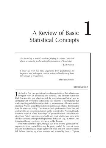
10INTERMEDIATE STATISTICSa bimodal distribution, and a normal distribution. The scores in a rectangular distribution are all about equally frequent or probable. Anexample of a rectangular distribution is the theoretical distribution representing the six possible scores that can be obtained by rolling a singlesix-sided die. In the case of a bimodal distribution, two distinct rangesof scores are more common than any other. A likely example of abimodal distribution would be the heights of the athletes attending theannual sports banquet for a very large high school that has only twosports teams: women’s gymnastics and men’s basketball. If this exampleseems a little contrived, it should. Bimodal distributions are relativelyrare, and they usually reflect the fact that a sample is composed of twomeaningful subsamples. The third distribution depicted in Figure 1.1 isthe most important. This is a normal distribution: a symmetrical, bellshaped distribution in which most scores cluster near the mean and inwhich scores become increasingly rare as they become increasinglydivergent from this mean. Many things that can be quantified are normally distributed. Distributions of height, weight, extroversion, selfesteem, and the age at which infants begin to walk are all examples ofapproximately normal distributions.The nice thing about the normal distribution is that if you know thata set of observations is normally distributed, this further improves yourability to describe the entire set of scores in the sample. More specifically,you can make some very good guesses about the exact proportion ofscores that fall within any given number of standard deviations (or fractions of a standard deviation) from the mean. As illustrated in Figure 1.2,about 68% of a set of normally distributed scores will fall within onestandard deviation of the mean. About 95% of a set of normally distributed scores will fall within two standard deviations of the mean, and wellover 99% of a set of normally distributed scores (99.8% to be exact) willfall within three standard deviations of the mean. For example, scores onmodern intelligence tests (such as the Wechsler Adult Intelligence Scale)are normally distributed, have a mean of 100, and have a standard deviation of 15. This means that about 68% of all people have IQs that fallbetween 85 and 115. Similarly, more than 99% of all people (again,99.8% of all people, to be more exact) should have IQs that fall between55 and 145.This kind of analysis can also be used to put a particular score orobservation into perspective (which is a first step toward making inferences from particular observations). For instance, if you know that a setof 400 scores on an astronomy midterm (a) approximates a normaldistribution, (b) has a mean of 70, and (c) has a standard deviation ofexactly 6, you should have a very good picture of what this entire set ofscores is like. And you should know exactly how impressed to be whenyou learn that your friend Amanda earned an 84 on the exam. Shescored 2.33 standard deviations above the mean, which means that sheprobably scored in the top 1% of the class. How could you tell this? By
Chapter 1 A Review of Basic Statistical Concepts11Figure 1.1 A Rectangular Distribution, a Bimodal Distribution, and a NormalDistributionMean 3.50Std. Dev. 1.871N 6Frequency1.00.80.60.40.20.01.002.003.004.00die rolls5.006.00Mean 71.50Std. Dev. 11.508N 24625Frequency2015105040.0050.0060.0070.0080.00new height100.00Mean 67.00Std. Dev. 4.671N ht in inches75.0080.00
12INTERMEDIATE STATISTICSFigure 1.2 Percentage of Scores in a Perfectly Normal Distribution Falling Within1, 2, and 3 Standard Deviations From the Mean99.8%95.4%68.2%0.40.30.234.1%0.10.1%0.0 3α2.1%34.1%13.6% 2α 1α2.1%13.6%µ1α2α0.1%3αSource: Image courtesy of Wikipedia.consulting a detailed table based on the normal distribution. Such atable would tell you that only about 2% of a set of scores are 2.33 standard deviations or more from the mean. And because the normal distribution is symmetrical, half of the scores that are 2.33 standarddeviations or more from the mean will be 2.33 standard deviations ormore below the mean. Amanda’s score was in the half of that 2% thatwas well above the mean. Translation: Amanda kicked butt on theexam.As you know if you have had any formal training in statistics, there ismuch more to descriptive statistics than what we have covered here. Forinstance, we skipped many of the specific measures of central tendencyand dispersion, and we didn’t describe all the possible kinds of distributions of scores. However, this overview should make it clear that descriptive statistics provide researchers with an enormously powerful tool fororganizing and simplifying data. At the same time, descriptive statistics areonly half of the picture. In addition to simplifying and organizing the datathey collect, researchers also need to draw conclusions about populationsfrom their sample data. That is, they need to move beyond the data themselves in the hopes of drawing general inferences about people. To do this,researchers rely on inferential statistics.
Chapter 1 A Review of Basic Statistical Concepts13Inferential StatisticsThe basic idea behind inferential statistical testing is that decisions aboutwhat to conclude from a set of research findings need to be made in alogical, unbiased fashion. One of the most highly developed forms of logicis mathematics, and statistical testing involves the use of objective, mathematical decision rules to determine whether an observed set of researchfindings is “real.” The logic of statistical testing is largely a reflection of theskepticism and empiricism that are crucial to the scientific method. Whenconducting a statistical test to aid in the interpretation of a set of experimental findings, researchers begin by assuming that the null hypothesis istrue. That is, they begin by assuming that their own predictions are wrong.In a simple, two-groups experiment, this would mean assuming that theexperimental group and the control group are not really different after themanipulation—and that any apparent difference between the two groupsis simply due to luck (i.e., to a failure of random assignment). After all,random assignment is good, but it is rarely perfect. It is always possi
Chapter 1 A Review of Basic Statistical Concepts 5 assembled a dream team of behavioral economists to help him get elected—and then to tackle the economic meltdown. This dream team relied not on classical economic models of what people ought to do but on empirical studi